4 Variability

An important characterization of a population is how spread out it is. One of the key measures of spread is variability. We measure population variability with the sample variance, or more often we consider the square root of both, called the standard deviation. The reason for taking the standard deviation is because that measure has the same units as the population. So if our population is a length measurement in meters, the standard deviation is in meters (whereas the variance is in meters squared).

Variability has many important uses in statistics. First, the population variance is itself an intrinsically interesting quantity that we want to estimate. Secondly, variability in our estimates is what makes them not imprecise. An important aspect of statistics is quantifying the variability in our estimates.

Variation:

\[Var(X) = E[(X-\mu)^2] = E[X^2]-E[X]^2\] Standard Deviation: \[\sigma = \sqrt{Var(X)}\]

Lets say that \(E[X] = 3.5\). \(E[X^2] = \frac{1}{6}(1^2)+\frac{1}{6}(2^2)+\frac{1}{6}(3^2)+\frac{1}{6}(4^2)+\frac{1}{6}(5^2)+\frac{1}{6}(6^2) = 15.17\)

\[Var(X) = E[X^2]-E[X]^2 = 15.17-3.5^2 = 2.92\]

4.1 Example For Coin Toss

\[E[X] = 0(1-p) + 1(p) = p\] \[E[X^2] = E[X] = p\] \[Var(X) = E[X^2]-E[X]^2 = p-p^2 = p(1-p)\] The variance, the population variance associated with the distribution given by the flip of a coin, a biased coin is exactly p times 1 minus p.

4.2 Sample Variance

\[S^2 = \frac{\sum_{i-1}(X_i-\bar{X})^2}{n-1}\]

Where:

\(n-1\) due to degrees of freedom
\(X_i\) observed observations
\(\bar{X}\) is the sample mean

The sample variance has its own distribution, as its value is decided by the data. This distribution has an expected value. As \(n-1\) increases, the sample variation will reduce, as it becomes more and more concentrated around the population variance.

The expected value of the sample mean \(E[\bar{X}]\) is \(\mu\) \[E[\bar{X}] = \mu\] The variance of the same mean \(Var(\bar{X})\) decreases with increasing sample size \(n\) as it approaches the value of the population variance \(\sigma^2\) \[Var(\bar{X}) = \frac{\sigma^2}{n}\]

The logical estimate of the mean is \[\frac{S^2}{n}\] The logical estimate of the standard error is \[\frac{S}{\sqrt{n}}\]

\(S\) the standard deviation, talks about how variable the population is. \(\frac{S}{\sqrt{n}}\) the standard error, talks about how variable averages of random samples of a size \(n\) from the population are.

4.3 Simulation Example

Standard normal have variance:1. This means that means of \(n\) standard normal have a standard deviation \(\frac{1}{\sqrt{n}}\).

nosim <- 1000
n <- 10
sd(apply(matrix(rnorm(nosim * n), nosim), 1, mean))

## [1] 0.3097786

1/sqrt(n)

## [1] 0.3162278

Poisson(4) have variance 4, means of random samples of \(n\) Poisson(4) have SD \(\frac{2}{\sqrt{n}}\)

nosim <- 1000
n <- 10
sd(apply(matrix(rpois(nosim * n, 4), nosim), 1, mean))

## [1] 0.6251164

2/sqrt(n)

## [1] 0.6324555

4.4 Data Example

library(UsingR);library(ggplot2)

data(father.son)

x <- father.son$sheight

n <- length(x)

hist(x)

var(x); var(x)/n; sd(x); sd(x)/sqrt(n)

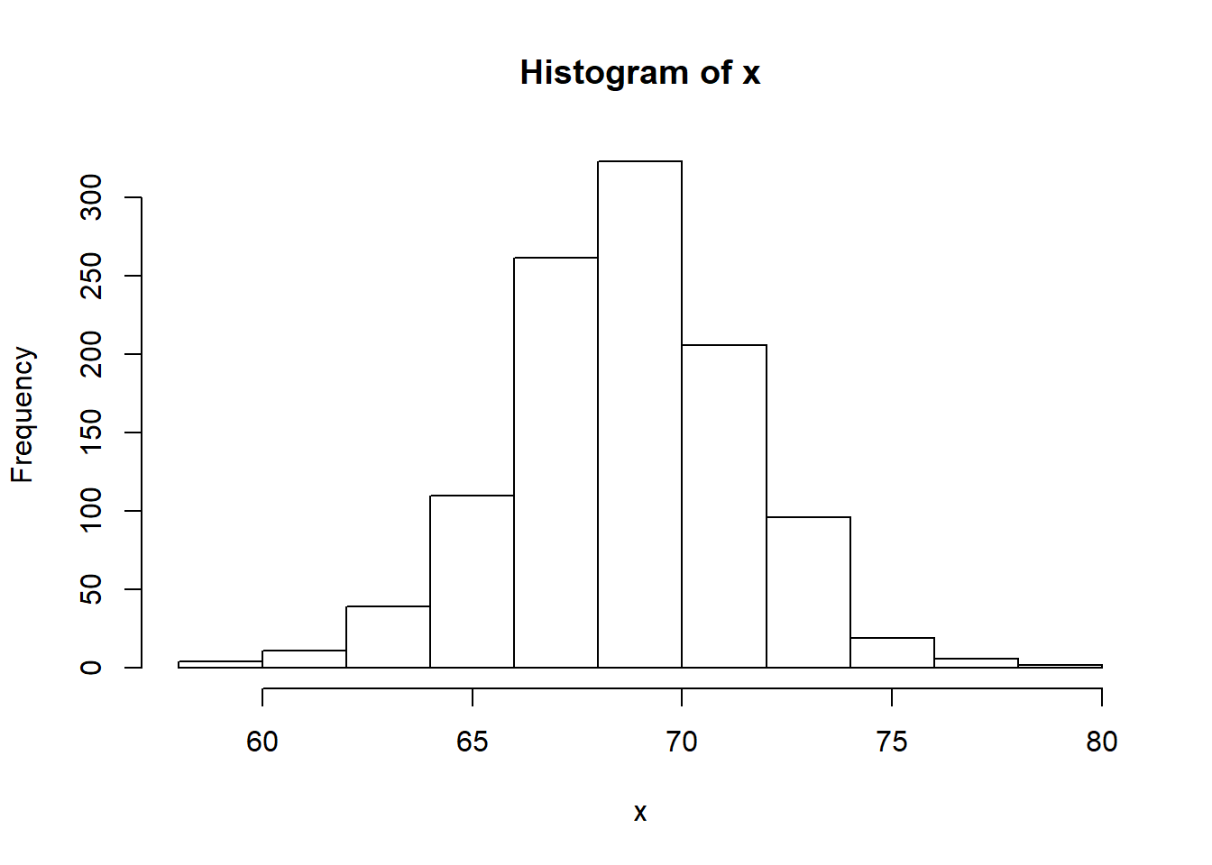
## [1] 7.922545

## [1] 0.0073493

## [1] 2.814702

## [1] 0.08572806