51 Predicting with Trees
51.1 Key Ideas
- Iteratively split variables into groups
- Evaluate “homogeneity” within each group
- Split again if necessary
Pros:
- Easy to interpret
- Better performance in non linear settings
Cons:
- Without pruning/cross-validation, this can lead to overfitting
- Harder to estimate uncertainty
- Results may be variable
51.2 The Basic Algorithm
- Start with all variables in one group
- Find the variable/split that best separates the outcomes
- Divide the data into two groups (“leaves”) on that split (“node”)
- Within each split, find the best variable/split that separates the outcomes
- Continue until the groups are too small or sufficiently homogeneous
51.3 Measures of Impurity
\[\hat{P}_{mk} = \frac{1}{N_m} \sum_{x_i~~ in~~ Leaf ~~m} \Bbb{I}(y_i = k)\]
Where:
- \(x_i\) is a particular observation on leaf \(m\).
- \(N_m\) is the number of objects that you can consider.
- \(y_i\) is the number of times that the class \(k\) appears in leaf \(m\).
- \(\hat{P}_{mk}\) is the probability that class \(k\) appears in leaf \(m\).
Misclassification Error: \[1-\hat{P}_{mk(m)}\]
- 0 = No entropy
- 0.5 = Perfect Entropy
Gini Index: \[\sum{}_{k \ne k} \hat{P}_{mk} \times \hat{P}_{mk~'} = \sum{}_{k=1}^K \hat{P}_{mk}(1- \hat{P}_{mk}) = 1 - \sum{}_{k=1}^K P^2_{mk}\]
\[1 - \sum{}_{k=1}^K P^2_{mk}\]
- 0 = No entropy
- 0.5 = Perfect Entropy
51.4 Example: Iris Data
# Load in the Data
data(iris); library(ggplot2); library(rattle)

# Examine the Data Labels
names(iris)
## [1] "Sepal.Length" "Sepal.Width" "Petal.Length" "Petal.Width" "Species"##
## setosa versicolor virginica
## 50 50 50# Create the training and testing sets
inTrain <- createDataPartition(y = iris$Species,
p = 0.7, list = FALSE)
training <- iris[inTrain, ]
testing <- iris[-inTrain, ]
dim(training); dim(testing)## [1] 105 5## [1] 45 5# Lets take a quick look at the distribution
ggplot(data = iris, aes(x = Petal.Width, y = Sepal.Width, col = Species)) +
geom_point() 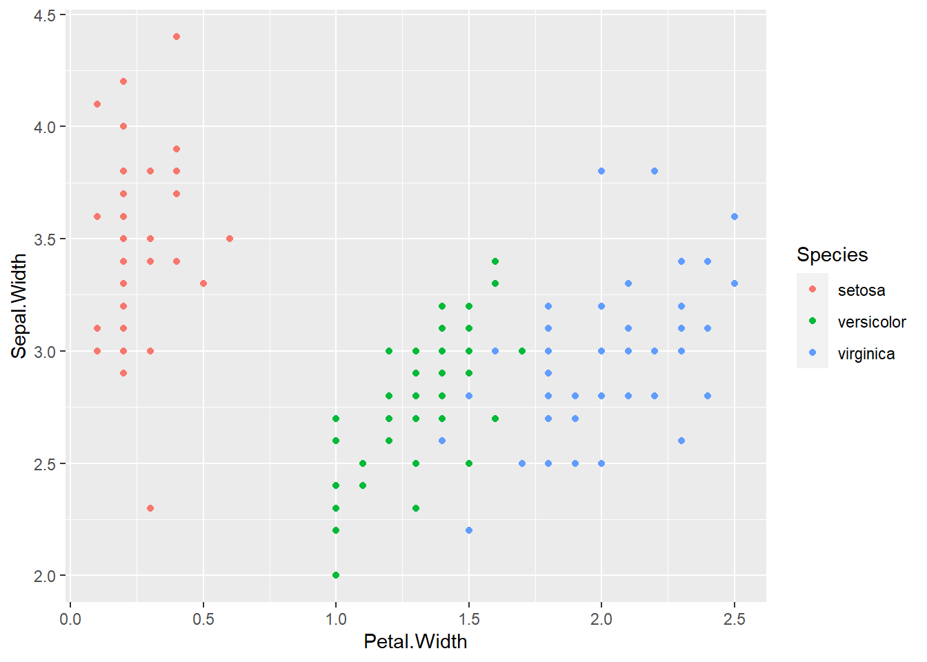
# We'll use the tree algorithm from the 'rpart' package bundled with caret to make the model
modFit <- train(Species ~. , method = "rpart", data = training)

# This package makes this shit to view, so if you want to have something that is easier to interpret, try using the C5.0 package or rattle
print(modFit$finalModel)
## n= 105
##
## node), split, n, loss, yval, (yprob)
## * denotes terminal node
##
## 1) root 105 70 setosa (0.3333333 0.3333333 0.3333333)
## 2) Petal.Length< 2.6 35 0 setosa (1.0000000 0.0000000 0.0000000) *
## 3) Petal.Length>=2.6 70 35 versicolor (0.0000000 0.5000000 0.5000000)
## 6) Petal.Length< 4.75 31 0 versicolor (0.0000000 1.0000000 0.0000000) *
## 7) Petal.Length>=4.75 39 4 virginica (0.0000000 0.1025641 0.8974359) *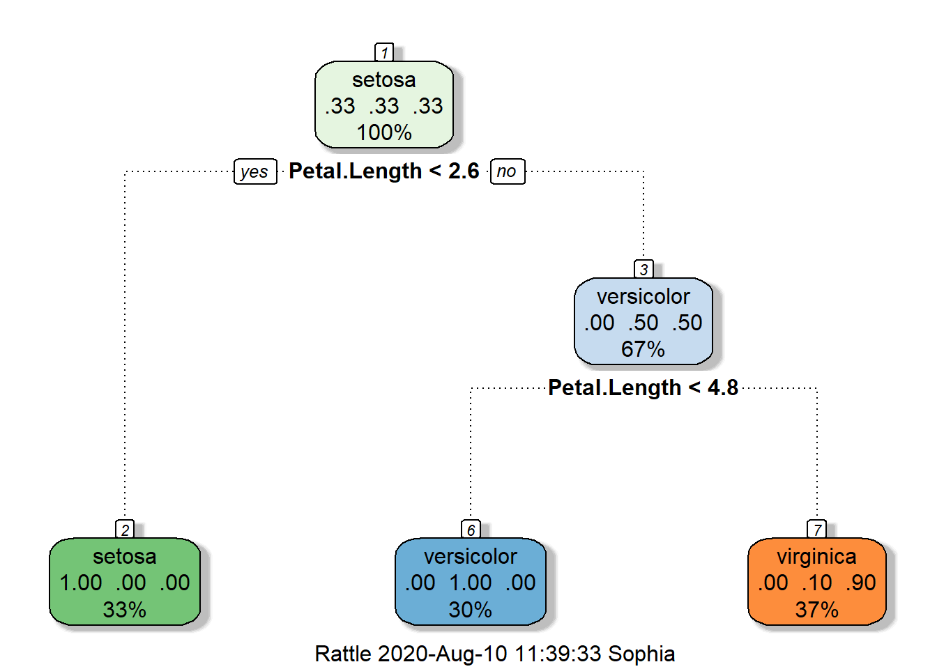
51.5 Notes:
- Classification trees are non-linear models
- As this is the case, they use interactions between variables
- Data transformations may be less important
- Trees can also be used for regression problems.
- More packages for building trees include:
party,rpart,c50andtree.