49 Predicting with Regression

49.1 Key Ideas

Fit a simple regression model
Plug in new covariates and multiply them by the coefficients
Useful when the linear model is (nearly) correct

Pros: * Easy to implement * easy to interpret

Cons: * Often poor performance on non-linear settings

49.2 Example: Geyser Eruptions

library(caret); data(faithful); set.seed(1234)
inTrain <- createDataPartition(y = faithful$waiting,
                               p = 0.5, list = FALSE)
trainFaith <- faithful[inTrain, ]; 
testFaith <- faithful[-inTrain, ]
head(trainFaith)

##    eruptions waiting
## 6      2.883      55
## 7      4.700      88
## 9      1.950      51
## 11     1.833      54
## 12     3.917      84
## 13     4.200      78

# Plot the waiting vs eruption data
ggplot(data = trainFaith, aes(x = waiting, y = eruptions, col = eruptions)) +
  geom_point() +
  geom_smooth( method = "lm")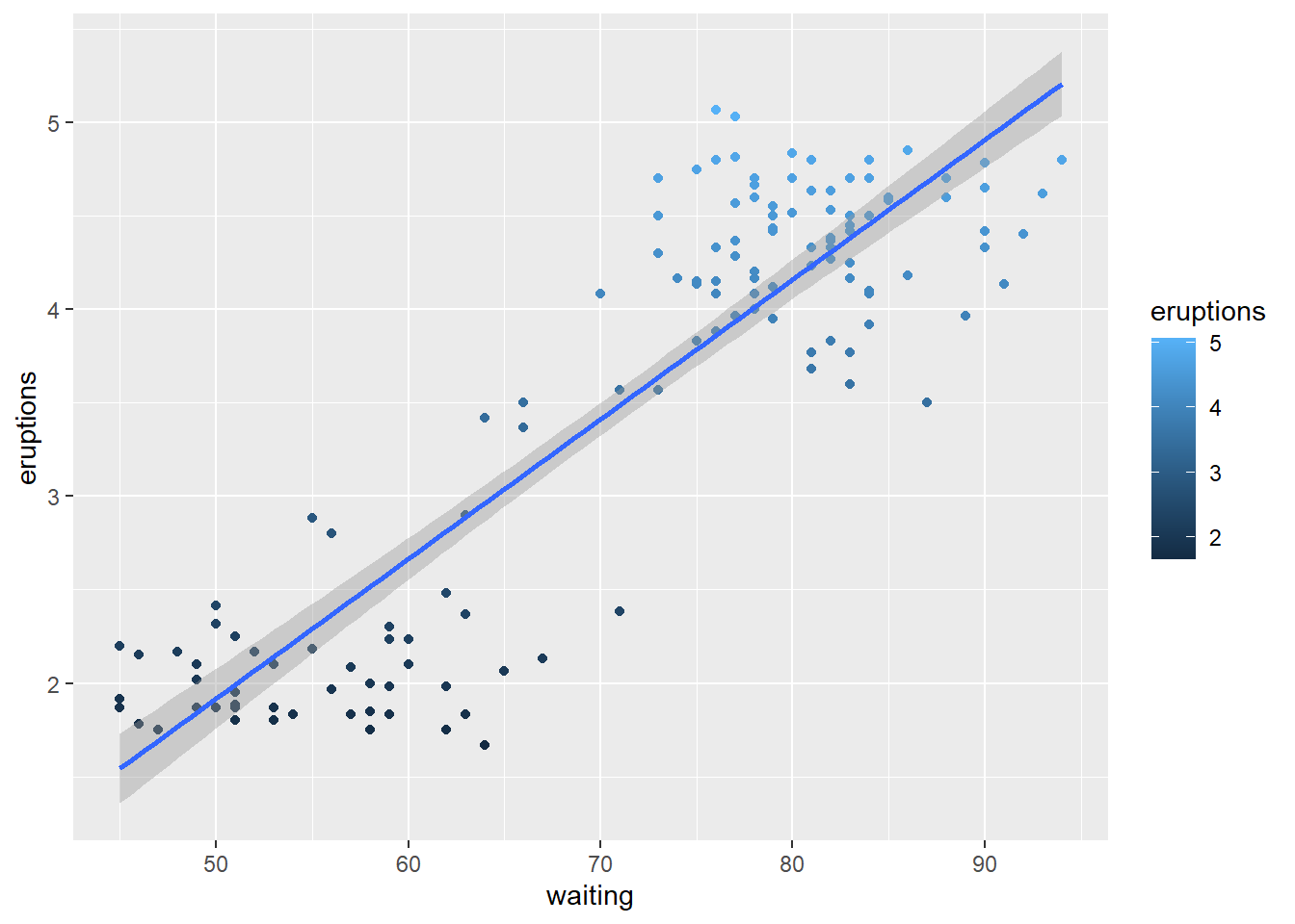

# Lets make an example linear model predicting eruptions using waiting time
lm1 <- lm(eruptions ~ waiting, data = trainFaith)
summary(lm1)

## 
## Call:
## lm(formula = eruptions ~ waiting, data = trainFaith)
## 
## Residuals:
##      Min       1Q   Median       3Q      Max 
## -1.29776 -0.37733  0.03967  0.35578  1.20490 
## 
## Coefficients:
##             Estimate Std. Error t value Pr(>|t|)    
## (Intercept) -1.82108    0.23306  -7.814  1.4e-12 ***
## waiting      0.07478    0.00323  23.148  < 2e-16 ***
## ---
## Signif. codes:  0 '***' 0.001 '**' 0.01 '*' 0.05 '.' 0.1 ' ' 1
## 
## Residual standard error: 0.5183 on 135 degrees of freedom
## Multiple R-squared:  0.7988, Adjusted R-squared:  0.7973 
## F-statistic: 535.8 on 1 and 135 DF,  p-value: < 2.2e-16

49.3 Predicting a New Value

So according to our model, what’s the predicted value of the eruption duration eruption given a waiting time of \(80\)?

Using the linear model: \[\hat{ED} = \hat{\beta_0} + \hat{\beta_1} WT\]

# with an example waiting time of 80, what is the expected value for eruption duration?
coef(lm1)[1] + coef(lm1)[2]*80

## (Intercept) 
##    4.161219

newdata <- data.frame(waiting = 80)
predict(lm1, newdata)

##        1 
## 4.161219

49.4 Plot Predictions: Training vs Test Set

par(mfrow = c(1,2))
plot(trainFaith$waiting, trainFaith$eruptions, col = "red", xlab = "Waiting", ylab = "Eruption Duration", main = "Training Set")
lines(trainFaith$waiting, predict(lm1), lwd = 3)

plot(testFaith$waiting, testFaith$eruptions, col = "blue", xlab = "Waiting", ylab = "Eruption Duration", main = "Predictions on the Test Set")
lines(testFaith$waiting, predict(lm1, newdata = testFaith), lwd = 3)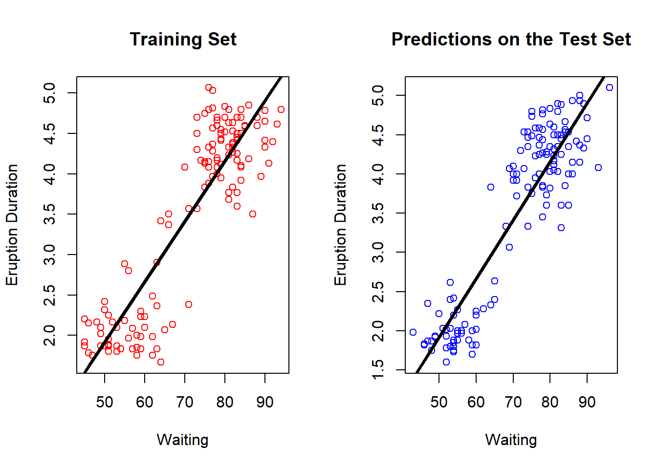

49.5 Get Training and Test set Errors

The measure of error for the linear model here will be \(RMSE\). This is the total difference between the fitted points and the actual points.

The \(RMSE\) for the test set is the exact same bench

# Caluculate the RMSE on the training set
sqrt(sum((lm1$fitted - trainFaith$eruptions)^2))

## [1] 6.021535

# Calculate the RMSE on the test set
sqrt(sum((predict(lm1, newdata = testFaith)-testFaith$eruptions)^2))

## [1] 5.509391

49.6 Prediction Intervals

Prediction intervals can be useful for looking at possible ranges that the values are likely to take. However, confidence intervals in general are probably more useful, this looks more or less intuitive going by the variation around the regression line.

Below we’ll use the regular plot(), matlines() and prediciton() functions, however this can also be done in the caret package.

# Calculate the prediction intervals! Using the linear model that we built on the training data
pred1 <- predict(lm1, newdata = testFaith, interval = "prediction")
ord <- order(testFaith$waiting)
plot(testFaith$waiting, testFaith$eruptions, pch = 8, col = "red")
matlines(testFaith$waiting[ord], pred1[ord, ], type = "l", col = c("blue","orange","orange"), lty = c(2,1,2), lwd = 3)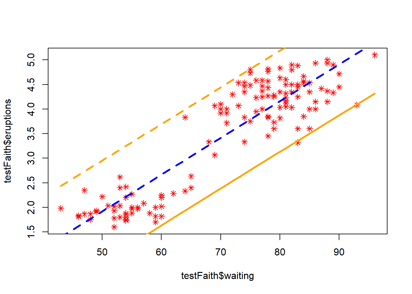

This process can also be done in the caret package.

# Create the model using the train function
modFit <- train(eruptions ~ waiting, data = trainFaith, method = "lm")

# The finalModel variable in the modFit object contains detailed information about the model created above, including the regression coefficients 
summary(modFit$finalModel)

## 
## Call:
## lm(formula = .outcome ~ ., data = dat)
## 
## Residuals:
##      Min       1Q   Median       3Q      Max 
## -1.29776 -0.37733  0.03967  0.35578  1.20490 
## 
## Coefficients:
##             Estimate Std. Error t value Pr(>|t|)    
## (Intercept) -1.82108    0.23306  -7.814  1.4e-12 ***
## waiting      0.07478    0.00323  23.148  < 2e-16 ***
## ---
## Signif. codes:  0 '***' 0.001 '**' 0.01 '*' 0.05 '.' 0.1 ' ' 1
## 
## Residual standard error: 0.5183 on 135 degrees of freedom
## Multiple R-squared:  0.7988, Adjusted R-squared:  0.7973 
## F-statistic: 535.8 on 1 and 135 DF,  p-value: < 2.2e-16