45 Plotting Predictors
# Load in the packages and the data
library(ISLR); library(ggplot2); library(psych); library(caret); data(Wage)
summary(Wage)
## year age maritl race
## Min. :2003 Min. :18.00 1. Never Married: 648 1. White:2480
## 1st Qu.:2004 1st Qu.:33.75 2. Married :2074 2. Black: 293
## Median :2006 Median :42.00 3. Widowed : 19 3. Asian: 190
## Mean :2006 Mean :42.41 4. Divorced : 204 4. Other: 37
## 3rd Qu.:2008 3rd Qu.:51.00 5. Separated : 55
## Max. :2009 Max. :80.00
##
## education region jobclass
## 1. < HS Grad :268 2. Middle Atlantic :3000 1. Industrial :1544
## 2. HS Grad :971 1. New England : 0 2. Information:1456
## 3. Some College :650 3. East North Central: 0
## 4. College Grad :685 4. West North Central: 0
## 5. Advanced Degree:426 5. South Atlantic : 0
## 6. East South Central: 0
## (Other) : 0
## health health_ins logwage wage
## 1. <=Good : 858 1. Yes:2083 Min. :3.000 Min. : 20.09
## 2. >=Very Good:2142 2. No : 917 1st Qu.:4.447 1st Qu.: 85.38
## Median :4.653 Median :104.92
## Mean :4.654 Mean :111.70
## 3rd Qu.:4.857 3rd Qu.:128.68
## Max. :5.763 Max. :318.34
## # Create the training and the testing sets
inTrain <- createDataPartition(y = Wage$wage, p = 0.7, list = FALSE)
training <- Wage[inTrain,]
testing <- Wage[-inTrain,]
dim(training); dim(testing)## [1] 2102 11## [1] 898 11# Feature plot? Looks like shit though...
featurePlot(x = training[, c("age", "education", "jobclass")], y = training$wage, plot = "pairs")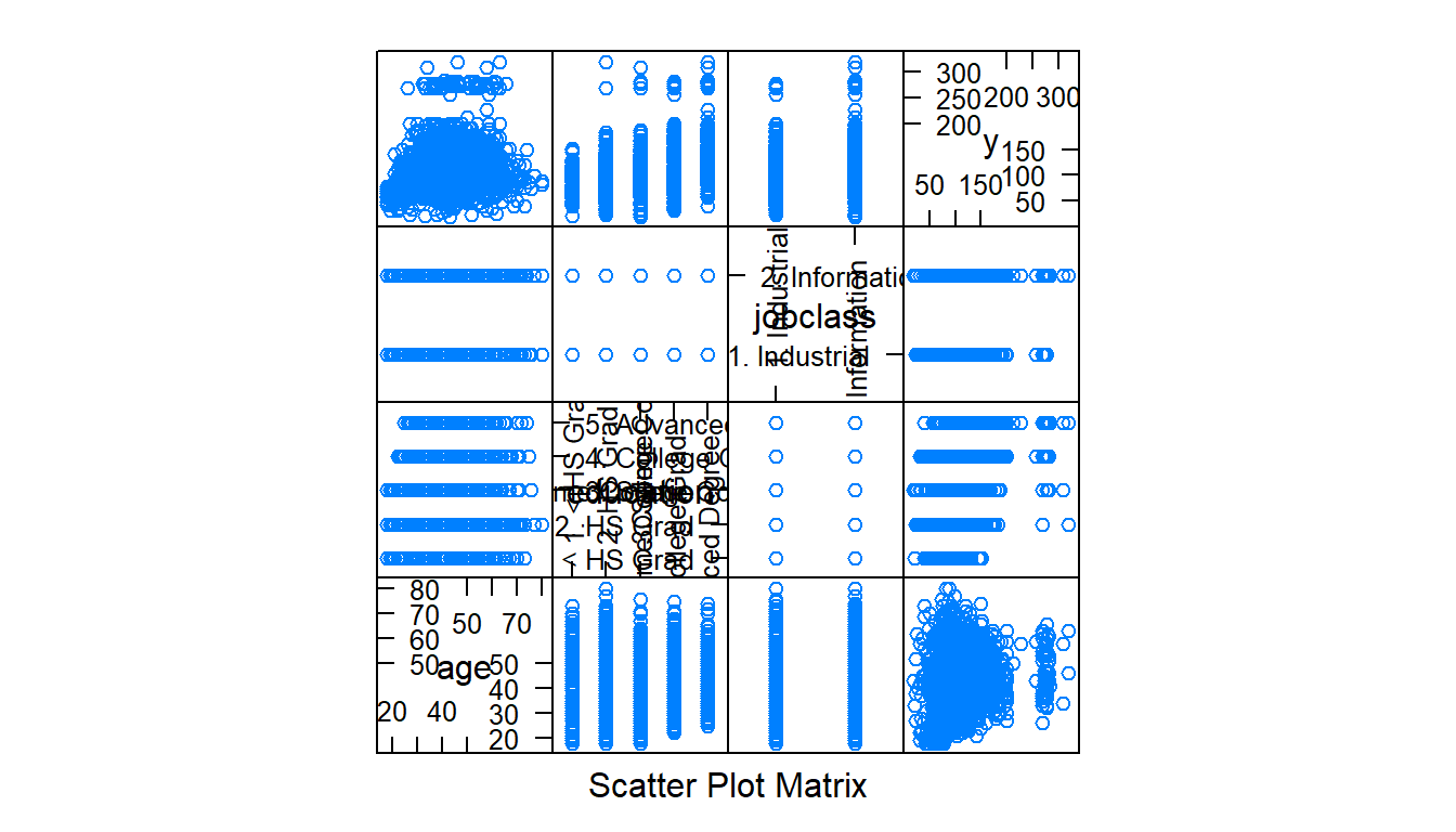
## `geom_smooth()` using formula 'y ~ x'
## `geom_smooth()` using formula 'y ~ x'
## `geom_smooth()` using formula 'y ~ x'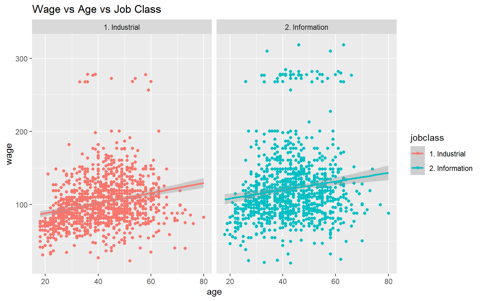
45.1 Making Factors with the Hmisc package
An easy way to automate the creation of factor variables with levels is to use the cut2() function from the Hmisc package. The ‘g’ argument tells the function how many levels you would like to have in your new factor.
# Load the Hmisc package
library(Hmisc)

# Use the cut2 function to break the data into 3 levels
cutWage <- cut2(training$wage, g = 3)

# Check that this works
table(cutWage)
## cutWage
## [ 20.1, 91.7) [ 91.7,118.9) [118.9,318.3]
## 704 726 672#
training$cutWage <- cutWage
ggplot(data = training, aes(x = cutWage, y = age, fill = cutWage)) +
geom_boxplot() +
geom_jitter(alpha = 0.15, pch =13, col = 'red') +
xlab("Wage Brackets") +
ylab("Age of Worker") +
ggtitle("Age of Worker vs Wage Braket")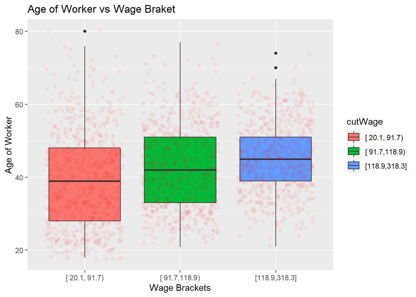
45.1.1 Making Tables
The factor variables created using the cut2() function can then be used to make tables and proportion tables that are useful for comparing other factors.
##
## cutWage         1. Industrial 2. Information
##   [ 20.1, 91.7)           459            245
##   [ 91.7,118.9)           375            351
## [118.9,318.3] 265 407##
## cutWage 1. Industrial 2. Information
## [ 20.1, 91.7) 0.6519886 0.3480114
## [ 91.7,118.9) 0.5165289 0.4834711
## [118.9,318.3] 0.3943452 0.6056548
45.2 Notes
- Only make plots on the training data.
- Need to look out for imbalance in the outcomes / predictors
- Need to look at outliers
- Need to look for groups of points not explained by a predictor
- Need to look for skewed variables.