16 Intro to Linear Regression
Regression models are the workhorse of data science. They are the most well described, practical and theoretically understood models in statistics. A data scientist well versed in regression models will be able to solve an incredible array of problems.
Perhaps the key insight for regression models is that they produce highly interpretable model fits. This is unlike machine learning algorithms, which often sacrifice interpretability for improved prediction performance or automation. These are, of course, valuable attributes in their own rights. However, the benefit of simplicity, parsimony and intrepretability offered by regression models (and their close generalizations) should make them a first tool of choice for any practical problem.
Note: View blog Simply Statistics
Linear regression is great for finding simple, meaningful relationships between variables and to figure out what assumptions are needed to generalize findings beyond the data in question.
16.1 Intro: Basic Least Squares
Lets look at the data used by Francis Galton in 1855 when he described the heights of children and parents using linear regression.
So lets look at the marginal distributions first:
- Parent distribution is all heterosexual couples.
- Correction for gender via multiplying female heights by 1.08.
- Overplotting is an issue from discretization.
library(UsingR); library(lmtest); library(psych);library(ggplot2); library(dplyr); data(galton); library(reshape2); long <- melt(galton)
g <- ggplot(long, aes(x = value, fill = variable))
g <- g + geom_histogram(colour = "black", binwidth = 1)
g <- g + facet_grid(.~ variable)
g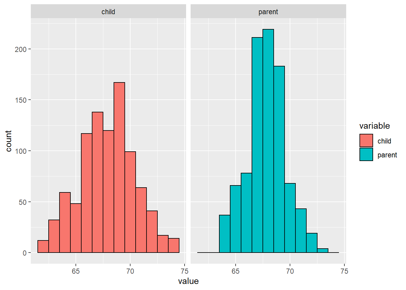
We’ve effectively broken the association between the two variables by not plotting a scatterplot, only looking at the marginal distributions of both the children and parents individually.
16.1.1 Finding the Middle via Least Squares
What would be the bets estimate at the child’s height given no information? We could just use the middle height.
Consider only the childrens heights:
How could one describe the “Middle”?
One definition, let \(Y_i\), be the height of child \(i\) for \(i=1,...,n=928\), then define the middle as the value of \(\mu\) the minimises: \[\sum_{i=1}^n (Y_i - \mu)^2\]
This is the physical centre of mass of the histogram.
The value of \(\mu\) that minimses the equation above is the mean. (\(\mu =\bar{Y}\))
library(UsingR)
library(manipulate)
library(ggplot2)
library(rpart)
library(rpart.plot)
data("galton")
myHist <- function(mu) {
  mse <- mean((galton$child - mu)^2)
  g <- ggplot(galton, aes(x = child)) + geom_histogram(fill = "salmon", colour = "black", binwidth = 1)
  g <- g + geom_vline(xintercept = mu, size = 3)
  g <- g + ggtitle(paste("mu = ", mu , ", MSE = ", round(mse, 2), sep = ""))
  g
}

myHist(68)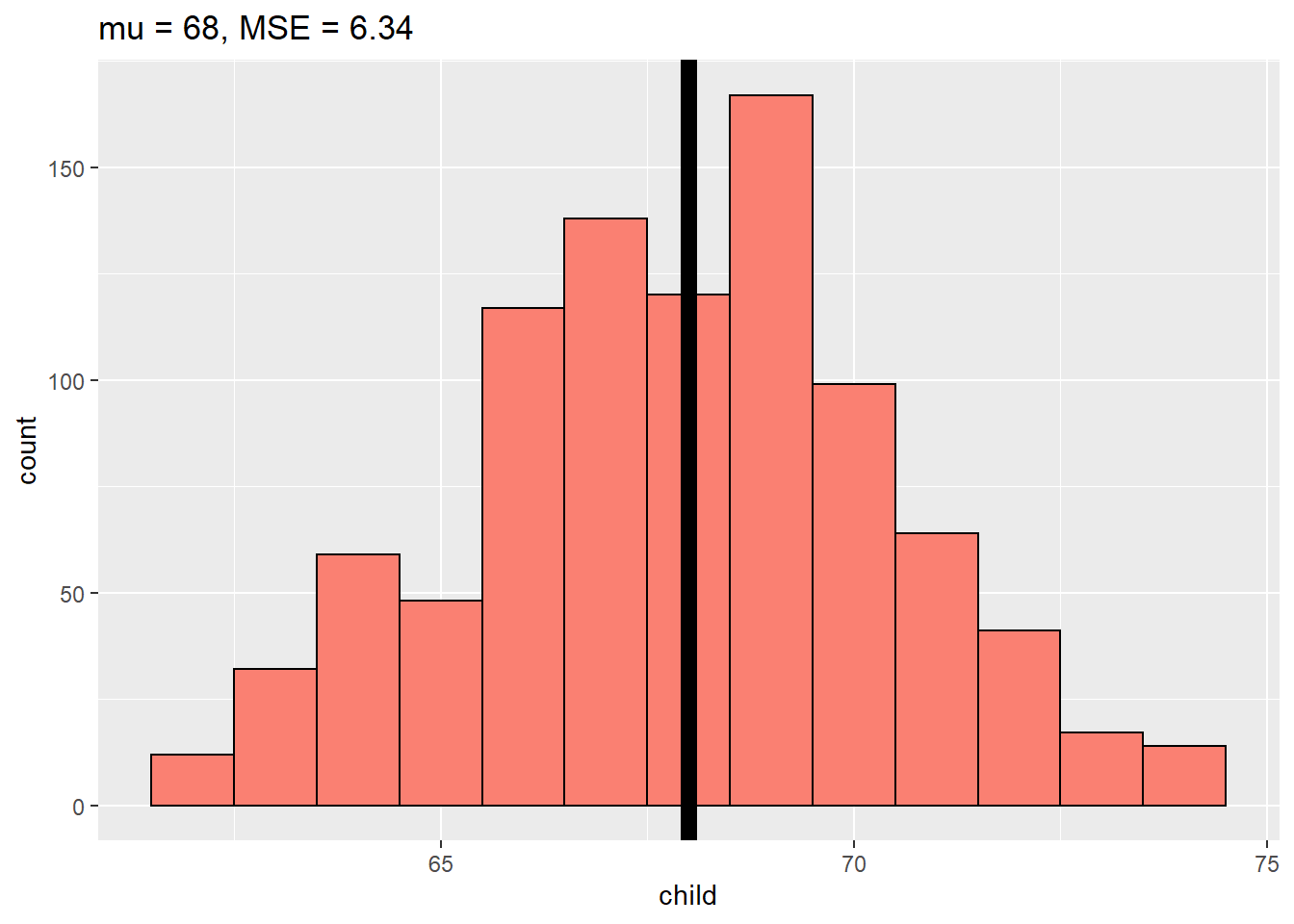
16.1.2 Proof that \(\bar{Y}\) is the minimiser
\(\sum_{i=1}^n (Y_i - \mu)^2 = \sum_{i=1}^n (Y_i - \bar{Y} + \bar{Y} - \mu)^2\)
\(= \sum_{i=1}^n (Y_i - \bar{Y})^2 + 2\sum_{i=1}^n (Y_i - \bar{Y})(\bar{Y}-\mu) + \sum_{i=1}^n(\bar{Y}-\mu)^2\)
\(= \sum_{i=1}^n (Y_i - \bar{Y})^2 +2(\bar{Y} - \mu) \sum_{i=1}^n(Y_i - \bar{Y}) + \sum_{i=1}^n(\bar{Y}-\mu)^2\)
\(= \sum_{i=1}^n (Y_i - \bar{Y})^2 +2(\bar{Y} - \mu) \sum_{i=1}^n(Y_i - n\bar{Y}) + \sum_{i=1}^n(\bar{Y}-\mu)^2\)
\(= \sum_{i=1}^n (Y_i - \bar{Y})^2 + \sum_{i=1}^n (\bar{Y} - \mu)^2\)
\(\ge \sum_{i=1}^n (Y_i - \bar{Y})^2\)
16.2 Comparing children’s heights to their parents’s heights
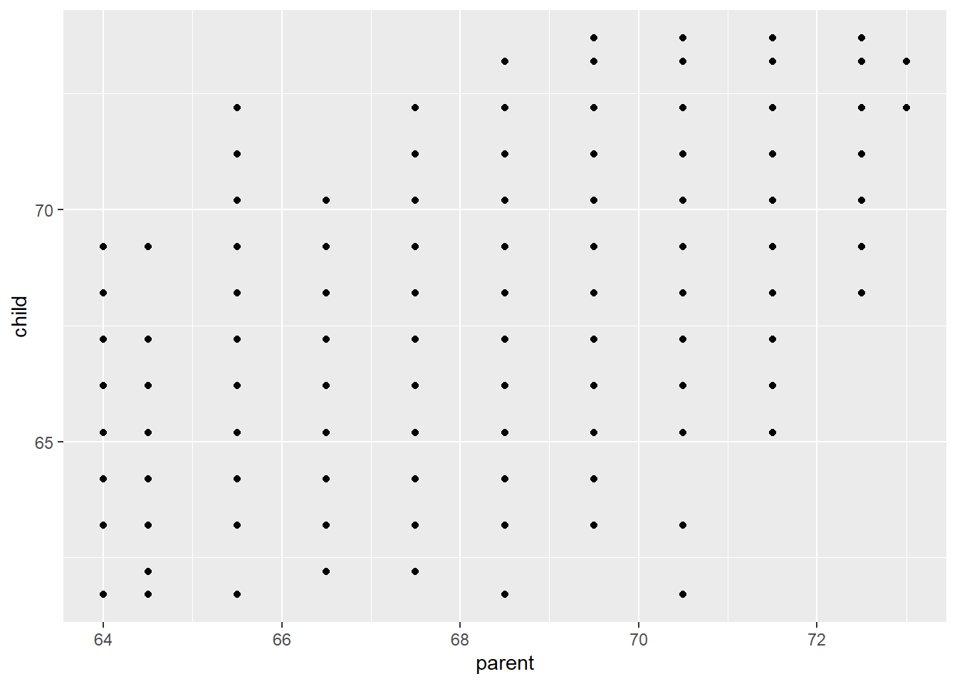
This plot sucks, as there’s a lot of overplotting, so we’ll need a way to visualise that…
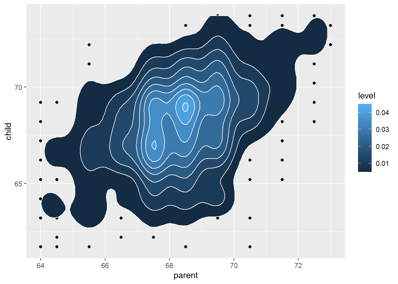
This plot does not loose this additional information.
16.3 Regression through the Origin
Suppose that we wanted to explain the children’s heights using the parents heights. Lets assume that we want to do that with a line. To make this task easy for now, lets do this with a line.
Suppose that \(Y_i\) are the cihldren’s heights and \(X_i\) are the heights of the parents.
Consider picking the slope \(\beta\) that minimises: \[\sum_{i=1}^n (Y_i - X_i \beta)^2\]
This uses the origin as a pivot point through which the line that minimises the su of the squared vertical distances of the points to the line is plotted.
In reality, we don’t want to do this, instead, set the origin as the centre of your data.
In the code chunk below we’re going to use the centred heights for both the children and the parents, hence I(child - mean(child)) ~ I(parent - mean(parent)) - 1 instead of just child ~ parent.
##
## Call:
## lm(formula = I(child - mean(child)) ~ I(parent - mean(parent)) -
##     1, data = galton)
##
## Coefficients:
## I(parent - mean(parent))
##                   0.6463
This gives us a coefficient (slope \(\beta\)) of 0.6463.