32 Poisson GLMs

Many data take the form of counts
- Calls to a call centre
- Number of flu cases in an area
- Number of cars that cross a bridge
Data may be also in the form of rates
- Percent of children passing a test
- Percent of hits to a website from a country
Linear regression with a transformation is an option here

32.1 Posison Distribution

The Poisson distribution is a useful model for counts and rates
Here a rate is count per some monitoring time
Some examples uses of the Poisson distribution
- Modeling web traffic hits
- Incidence rates
- Approximating binomial probabilities with small \(p\) and large \(n\)
- Analyzing contigency table data

32.2 Poisson Mass Function

\(X \sim Poisson(t\lambda)\) if \[ P(X = x) = \frac{(t\lambda)^x e^{-t\lambda}}{x!} \] For \(x = 0, 1, \ldots\).
The mean of the Poisson is \(E[X] = t\lambda\), thus \(E[X / t] = \lambda\)
The variance of the Poisson is \(Var(X) = t\lambda\).
The Poisson tends to a normal as \(t\lambda\) gets large.

par(mfrow = c(1, 3))
plot(0 : 10, dpois(0 : 10, lambda = 2), type = "h", frame = FALSE)
plot(0 : 20, dpois(0 : 20, lambda = 10), type = "h", frame = FALSE)
plot(0 : 200, dpois(0 : 200, lambda = 100), type = "h", frame = FALSE)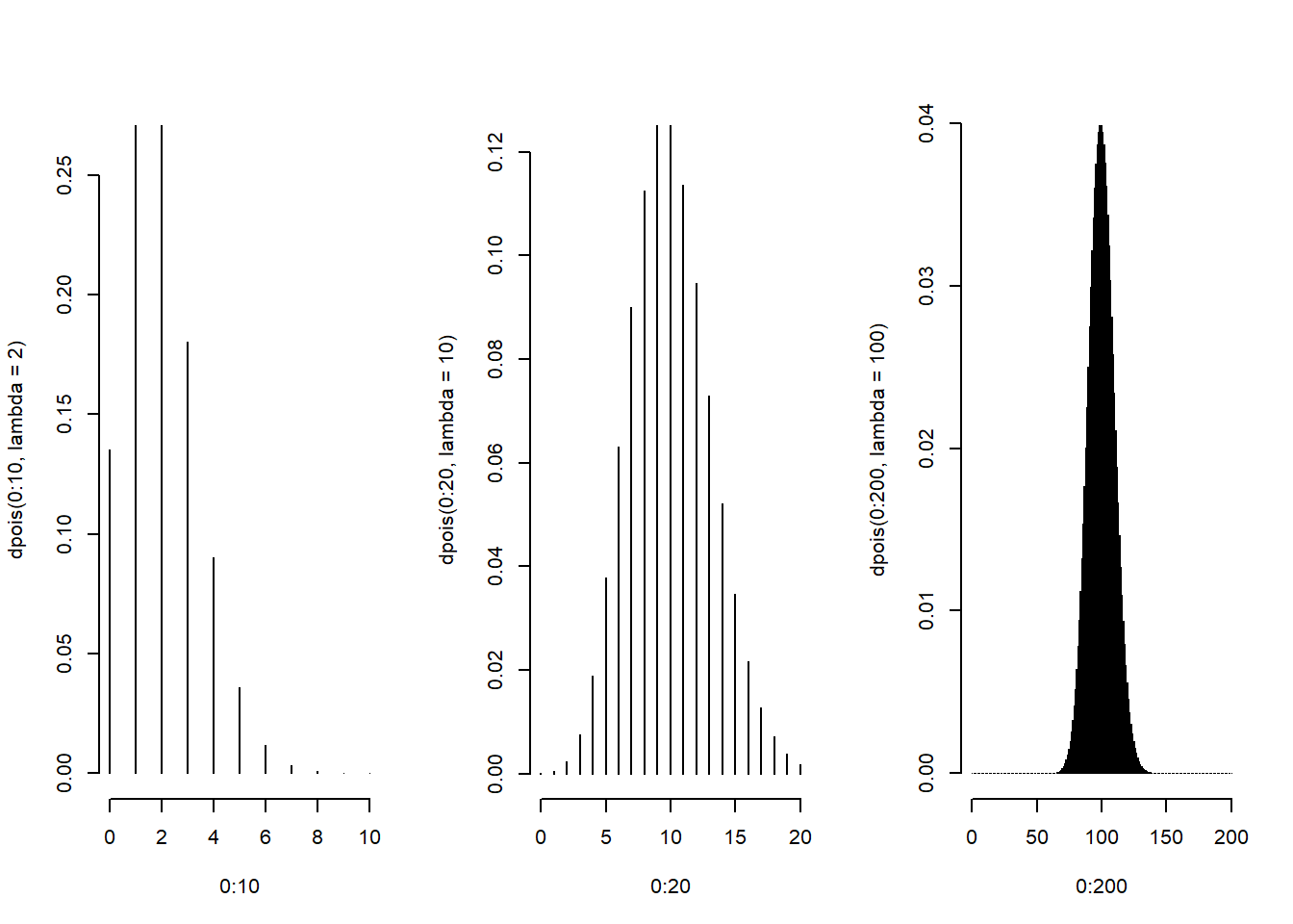

x <- 0 : 10000; lambda = 3
mu <- sum(x * dpois(x, lambda = lambda))
sigmasq <- sum((x - mu)^2 * dpois(x, lambda = lambda))
c(mu, sigmasq)

## [1] 3 3

32.3 Linear regression

\[ NH_i = b_0 + b_1 JD_i + e_i \]

\(NH_i\) - number of hits to the website

\(JD_i\) - day of the year (Julian day)

\(b_0\) - number of hits on Julian day 0 (1970-01-01)

\(b_1\) - increase in number of hits per unit day

\(e_i\) - variation due to everything we didn’t measure

Taking the natural log of the outcome has a specific interpretation.
Consider the model

\[ \log(NH_i) = b_0 + b_1 JD_i + e_i \]

\(NH_i\) - number of hits to the website

\(JD_i\) - day of the year (Julian day)

\(b_0\) - log number of hits on Julian day 0 (1970-01-01)

\(b_1\) - increase in log number of hits per unit day

\(e_i\) - variation due to everything we didn’t measure

32.4 Exponentiating Coefficients

\(e^{E[\log(Y)]}\) geometric mean of \(Y\).
- With no covariates, this is estimated by: \[e^{\frac{1}{n}\sum_{i=1}^n \log(y_i)} = (\prod_{i=1}^n y_i)^{1/n}\]
When you take the natural log of outcomes and fit a regression model, your exponentiated coefficients estimate things about geometric means.
\(e^{\beta_0}\) estimated geometric mean hits on day 0
\(e^{\beta_1}\) estimated relative increase or decrease in geometric mean hits per day
There’s a problem with logs with you have zero counts, adding a constant works

32.5 Linear vs Poisson

Linear

\[ NH_i = b_0 + b_1 JD_i + e_i \]

\[ E[NH_i | JD_i, b_0, b_1] = b_0 + b_1 JD_i\]

Poisson/log-linear

\[ \log\left(E[NH_i | JD_i, b_0, b_1]\right) = b_0 + b_1 JD_i \]

\[ E[NH_i | JD_i, b_0, b_1] = \exp\left(b_0 + b_1 JD_i\right) \]

32.5.1 Multiplicitive Differences

\[ E[NH_i | JD_i, b_0, b_1] = \exp\left(b_0 + b_1 JD_i\right) \]

\[ E[NH_i | JD_i, b_0, b_1] = \exp\left(b_0 \right)\exp\left(b_1 JD_i\right) \]

32.6 Rates

\[ E[NHSS_i | JD_i, b_0, b_1]/NH_i = \exp\left(b_0 + b_1 JD_i\right) \]

\[ \log\left(E[NHSS_i | JD_i, b_0, b_1]\right) - \log(NH_i) = b_0 + b_1 JD_i \]

\[ \log\left(E[NHSS_i | JD_i, b_0, b_1]\right) = \log(NH_i) + b_0 + b_1 JD_i \]