46 Preprocessing
46.1 Why Preprocess?
From the SPAM data below, it is evident that preprocessing is needed in order to prevent our machine learning models from being tricked by the hugely varied data.
set.seed(123)

# Use data partition functions to create the training and testing sets
inTrain <- createDataPartition(y = spam$type,
                               p = 0.75,
                               list=FALSE)
training <- spam[inTrain, ]
testing <- spam[-inTrain, ]

# Lets plot a variable to see it's distibution
hist(training$capitalAve, main="", xlab = "Average capital run length")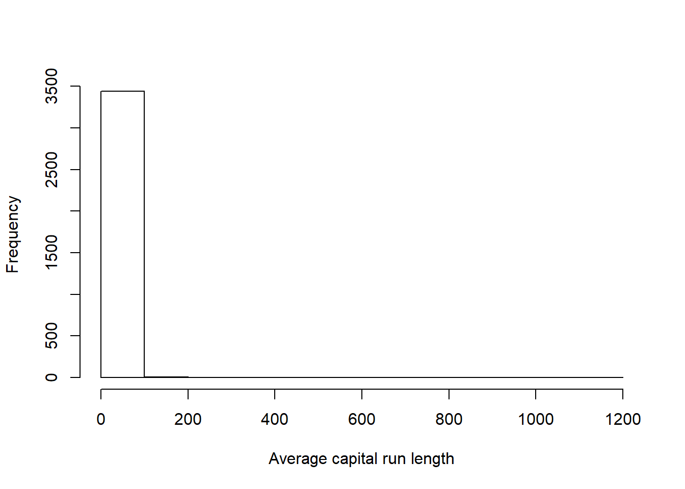
# Hard to see the distribution as it's so extremely skewed, lets try taking the log of the same variable
hist(log10(training$capitalAve), main="", xlab = "Log 10 Average capital run length")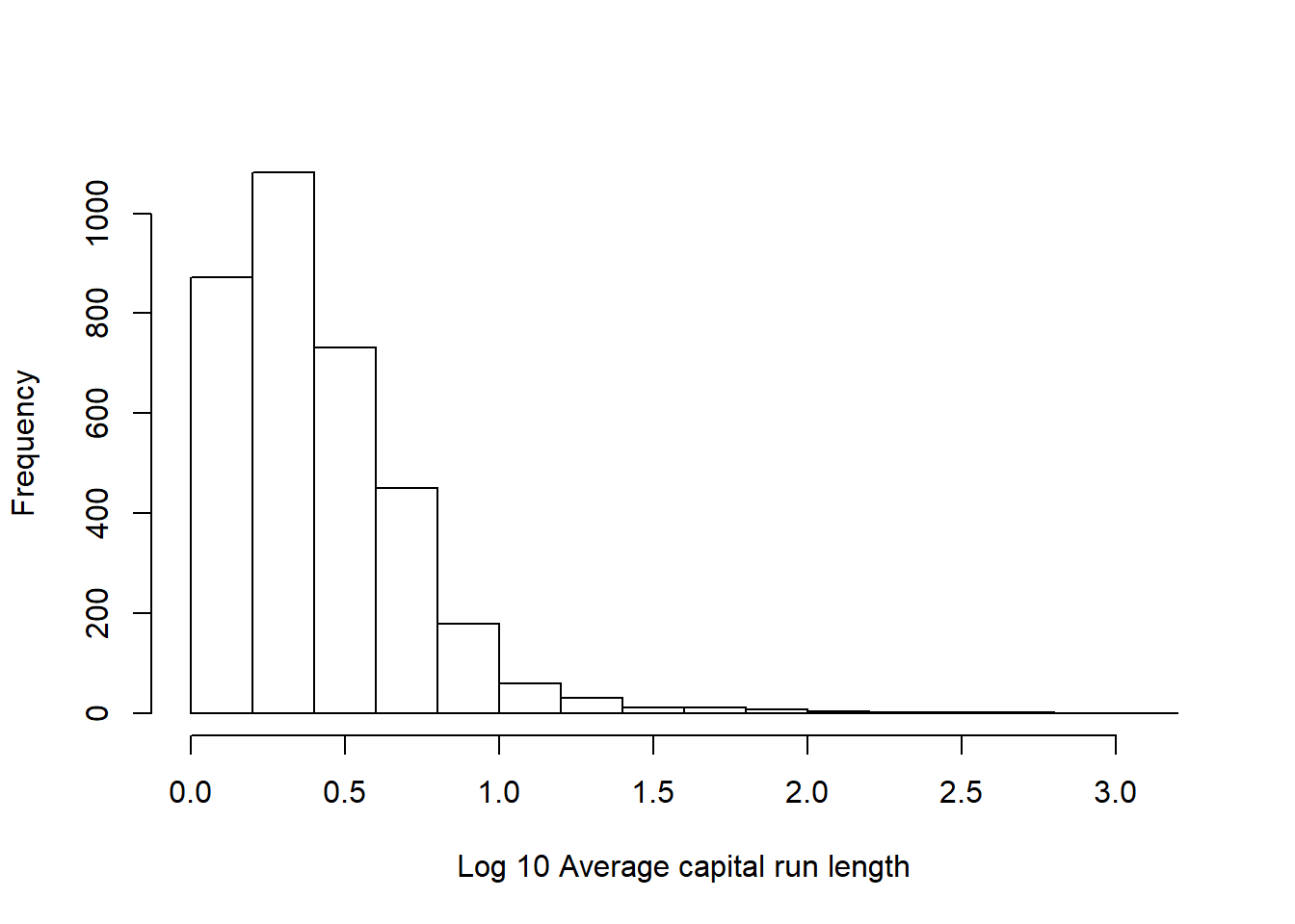
##     Min.  1st Qu.   Median     Mean  3rd Qu.     Max.
## 1.000 1.575 2.277 4.864 3.714 1102.500## [1] 27.8017346.2 Standardising
One way of getting around this is to standardise the data. Standardise the data by : \[Standardised~~ Data ~=~ \frac{Sample - Mean(Sample)}{Sd(Sample)}\] Just be sure not to forget that if you’re standardising the training set, you also have to standardise the testing set otherwise you’re not in for a good time.
trainCapAve <- training$capitalAve

# Standardise the data
trainCapAveS <- (trainCapAve - mean(trainCapAve))/sd(trainCapAve)

# Check it works still
mean(trainCapAveS)
## [1] 9.854945e-18## [1] 1# Dont forget to also standardise the test set
testCapAve <- testing$capitalAve
testCapAveS <- (testCapAve - mean(testCapAve))/sd(testCapAve)
# Check it works still
mean(testCapAveS)## [1] 8.507133e-18## [1] 146.2.1 Using the preProcess function
A lot of the standard preprocessing techniques can be done automatically by using the preProcess() function from the caret package. The ‘method’ argument tells the function what preprocessing you would like to be done, the ‘center’ and ‘scale’ arguments are listed below.
preObj <- preProcess(training[,-58], method = c("center", "scale"))
trainCapAveS <- predict(preObj, training[, -58])$capitalAve
mean(trainCapAveS)
## [1] 8.680584e-18## [1] 1## [1] 0.04713308## [1] 1.486708The preProcessing() function can also be passed as an argument to the train() function.
modelFit <- train(type ~., data = training,
                  preProcess = c("center", "scale"),
                  method = "glm")
modelFit
## Generalized Linear Model
##
## 3451 samples
## 57 predictor
## 2 classes: 'nonspam', 'spam'
##
## Pre-processing: centered (57), scaled (57)
## Resampling: Bootstrapped (25 reps)
## Summary of sample sizes: 3451, 3451, 3451, 3451, 3451, 3451, ...
## Resampling results:
##
## Accuracy Kappa
## 0.9191452 0.828881846.3 Standardising: Box-Cox Transforms
Standarising helps to remove really strongly biased predictors or predictors with really high variability. The Box-Cox transforms take a set of continuous data and try to make them look like normal data by estimating a specific set of parameters using MLE (Maximum likelihood estimation). Note that the Box-Cox transformations still encounter problems with 0 value samples. (There is still a fairly large stack of them in the histogram plot below)
# Preprocess you data using Box-Cox transformation
preObj <- preProcess(training[, -58], method = c("BoxCox"))

# Predict using the preprocessed data
trainCapAveS <- predict(preObj, training[, -58])$capitalAve
testCapAveS <- predict(preObj, testing[, -58])$capitalAve

par(mfrow = c(2,2))

# Plot theresulting data
hist(trainCapAveS)
qqnorm(trainCapAveS)
hist(testCapAveS)
qqnorm(testCapAveS)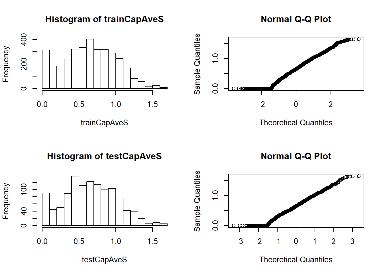
46.4 Standardising: Imputing Data
Often you will be forced to work with data sets that contain missing data. Predictive algorithms will usually fail in these cases. One way around this, is to impute the missing data. In this case we will use K-Nearest Neighbors Imputation to input the missing data. It is important to note that this is a random process, so it is important to set the seed to ensure reproducible results.
library(RANN)

set.seed(123)

# Use data partition functions to create the training and testing sets
inTrain <- createDataPartition(y = spam$type,
                               p = 0.75,
                               list=FALSE)
training <- spam[inTrain, ]
testing <- spam[-inTrain, ]

# First, start by making some values NA
training$capAve <- training$capitalAve
selectNA <- rbinom(dim(training)[1], size =1, prob = 0.05)==1
training$capAve[selectNA] <- NA

# Now impute and standardise the data
preObj <- preProcess(training[,-58], method = "knnImpute")
capAve <- predict(preObj, training[, -58])$capAve

# Standardise the true values
capAveTruth <- training$capitalAve
capAveTruth <- (capAveTruth - mean(capAveTruth))/sd(capAveTruth)

# Lets see if this checks out
quantile(capAve - capAveTruth)
## 0% 25% 50% 75% 100%
## -2.3541187775 0.0006568801 0.0018603563 0.0024353679 0.2137068700## 0% 25% 50% 75% 100%
## -2.354118777 -0.025095587 0.002530341 0.012163980 0.213706870## 0% 25% 50% 75% 100%
## -0.8630004021 0.0007258579 0.0018568190 0.0024090345 0.0028578816