26 Model Selection
“How do we chose what variables to include in a regression model?”. Sadly, no single easy answer exists and the most reasonable answer would be “It depends.”. These concepts bleed into ideas of machine learning, which is largely focused on high dimensional variable selection and weighting. In the following lectures we cover some of the basics and, most importantly, the consequences of over- and under-fitting a model.
26.1 Multiple Variables
- In modeling, our interest lies in parsimonious, interpretable representations of our data.
- A model is a lense through which to look at your data, under this philosophy, what’s the right model?
- The right model is really any model that connects the data to a true parsimonious statement about what you’re studying.
- The right model should present the same data in a way that highlights the certain thing that you’re looking for.
- Including variables that we shouldn’t have, increases standard errors of the regression variables. (Adds bias)
- Adding additional regressors that we don’t need can act like standard errors in the way that even if they do not induce bias, they will still inflate the standard errors of more relevent regressors.
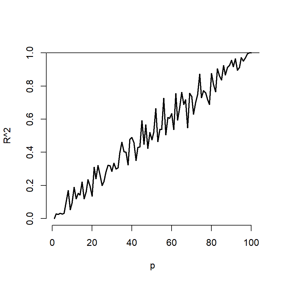
- \(R^2\) will always increase monotonically, as more regressors are added. Even adding bullshit ones.
- The squared standard error decreases monotonically as more regressors are included also.
For simulations, as the number of variables included equals increases to \(n=100\). No actual regression relationship exist in any simulation:
26.2 Variance Inflation
n <- 100; nosim <- 1000
x1 <- rnorm(n); x2 <- rnorm(n); x3 <- rnorm(n);
betas <- sapply(1 : nosim, function(i){
  y <- x1 + rnorm(n, sd = .3)
  c(coef(lm(y ~ x1))[2],
    coef(lm(y ~ x1 + x2))[2],
    coef(lm(y ~ x1 + x2 + x3))[2])
})
round(apply(betas, 1, sd), 5)
## x1 x1 x1
## 0.02972 0.02969 0.02974- Notice variance inflation was much worse when we included a variable that
was highly related to
x1. - We don’t know \(\sigma\), so we can only estimate the increase in the actual standard error of the coefficients for including a regressor.
- However, \(\sigma\) drops out of the relative standard errors. If one sequentially adds variables, one can check the variance (or sd) inflation for including each one.
- When the other regressors are actually orthogonal to the regressor of interest, then there is no variance inflation.
- The variance inflation factor (VIF) is the increase in the variance for the ith regressor compared to the ideal setting where it is orthogonal to the other regressors.
- (The square root of the VIF is the increase in the sd …)
- Remember, variance inflation is only part of the picture. We want to include certain variables, even if they dramatically inflate our variance.
26.3 Variable Inclusion and Exclusion
- (Known Knowns) - Regressors that we know that we should check to include in the model and have.
- (Known Unknowns) - Regressors that we would like to include in the model but don’t have access to.
- (Unknown Unknowns) - Regressors that we don;t even know about, that we should have included in the model.
26.4 Predicting Medical Expenses using MLR
# Our models dependant variable is "expenses" which measures medical costs each person charged to the insurance agency for the year.
insurance <- read.csv(file = "insurance.csv")
str(insurance)
## 'data.frame': 1338 obs. of 7 variables:
## $ age : int 19 18 28 33 32 31 46 37 37 60 ...
## $ sex : Factor w/ 2 levels "female","male": 1 2 2 2 2 1 1 1 2 1 ...
## $ bmi : num 27.9 33.8 33 22.7 28.9 ...
## $ children: int 0 1 3 0 0 0 1 3 2 0 ...
## $ smoker : Factor w/ 2 levels "no","yes": 2 1 1 1 1 1 1 1 1 1 ...
## $ region : Factor w/ 4 levels "northeast","northwest",..: 4 3 3 2 2 3 3 2 1 2 ...
## $ charges : num 16885 1726 4449 21984 3867 ...Before building our model, it is important to check for normality in our data. Although linear regression does not require a normally distributed dependant variable, the model often fits better when that is the case:
##    Min. 1st Qu.  Median    Mean 3rd Qu.    Max.
##    1122    4740    9382   13270   16640   63770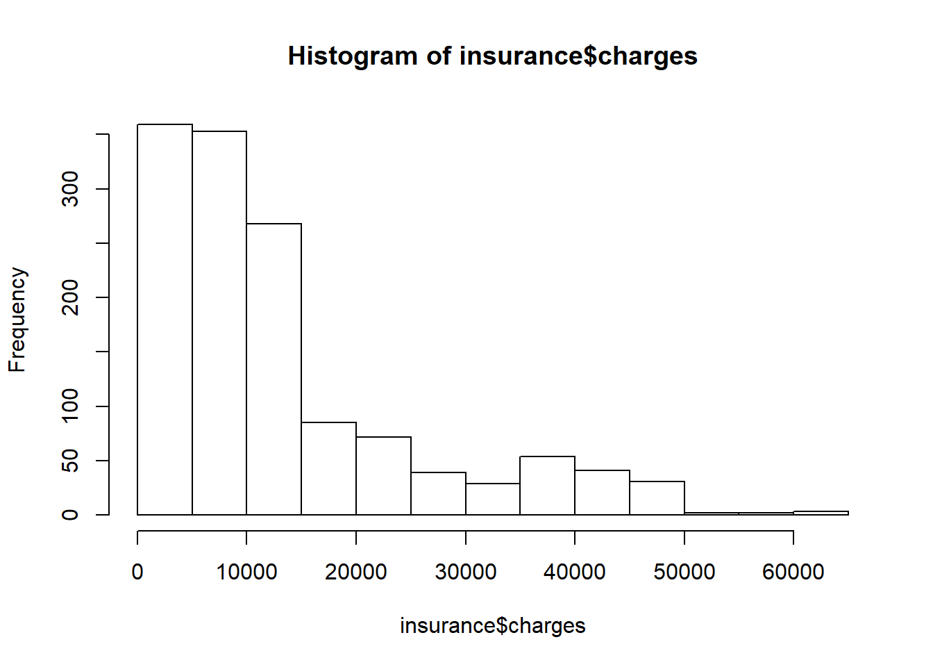
As we can see, the distribution is righ-skewed, with a most people paying betwwen 0 and 15,000 per year. Although this isn’t ideal, we can use this information to build a better model in the future.
Before we can begin to address this issue, we have to change some of the factor variables into numerics. The sex and smoker variables are coded as factors. The region factor has 4 levels, so lets check how those are distributed as well.
##
## northeast northwest southeast southwest
##       324       325       364       325
Lets see how the variables in the data set relate to eachother, these relationships can help to detect confounding variables.
##                age       bmi   children    charges
## age      1.0000000 0.1092719 0.04246900 0.29900819
## bmi      0.1092719 1.0000000 0.01275890 0.19834097
## children 0.0424690 0.0127589 1.00000000 0.06799823
## charges  0.2990082 0.1983410 0.06799823 1.00000000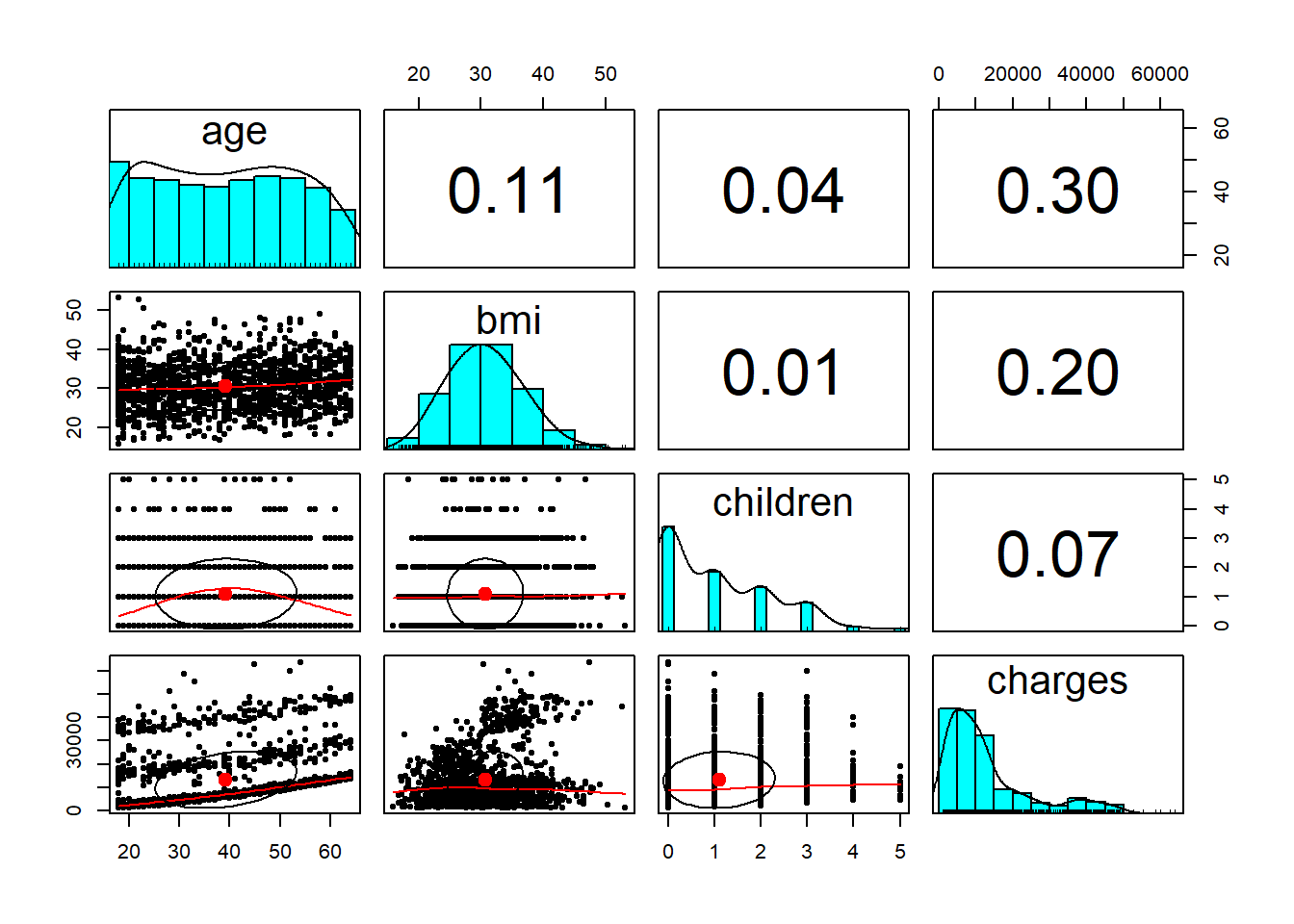
From the correlation matrix above, none of the dependant variables have any strong relationships to eachother, apart from the bmi and age variables sharing a weak positive trend.
Time to fit a linear regression model to the data.
##
## Call:
## lm(formula = charges ~ ., data = insurance)
##
## Residuals:
##      Min       1Q   Median       3Q      Max
## -11304.9  -2848.1   -982.1   1393.9  29992.8
##
## Coefficients:
##                 Estimate Std. Error t value Pr(>|t|)
## (Intercept)     -11938.5      987.8 -12.086  < 2e-16 ***
## age                256.9       11.9  21.587  < 2e-16 ***
## sexmale           -131.3      332.9  -0.394 0.693348
## bmi                339.2       28.6  11.860  < 2e-16 ***
## children           475.5      137.8   3.451 0.000577 ***
## smokeryes        23848.5      413.1  57.723  < 2e-16 ***
## regionnorthwest   -353.0      476.3  -0.741 0.458769
## regionsoutheast  -1035.0      478.7  -2.162 0.030782 *
## regionsouthwest   -960.0      477.9  -2.009 0.044765 *
## ---
## Signif. codes:  0 '***' 0.001 '**' 0.01 '*' 0.05 '.' 0.1 ' ' 1
##
## Residual standard error: 6062 on 1329 degrees of freedom
## Multiple R-squared:  0.7509, Adjusted R-squared:  0.7494
## F-statistic: 500.8 on 8 and 1329 DF,  p-value: < 2.2e-16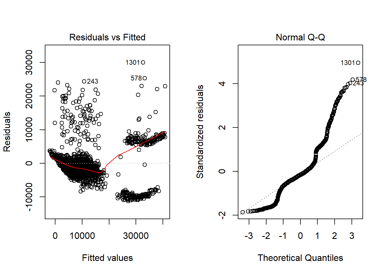
The coefficients from our model tell us that for every additional year of age, the yearly expenses on average increase by $257. Our model also tells us that males on average pay $131 per year less than females. Similarly, for every additional child, there is an associated increase in expenses of $476 and for every unit increase in BMI, the charges increase by $339. The largest increase by far however, is wheather or not the individual is a smoker, as there is an increase on average of $23,848 per year for smokers.
26.4.1 Evaluating Model Performance
##
## Call:
## lm(formula = Fertility ~ Agriculture * factor(CatholicBin), data = swiss)
##
## Residuals:
##     Min      1Q  Median      3Q     Max
## -28.840  -6.668   1.016   7.092  20.242
##
## Coefficients:
##                                  Estimate Std. Error t value Pr(>|t|)
## (Intercept)                      62.04993    4.78916  12.956   <2e-16 ***
## Agriculture                       0.09612    0.09881   0.973    0.336
## factor(CatholicBin)1              2.85770   10.62644   0.269    0.789
## Agriculture:factor(CatholicBin)1  0.08914    0.17611   0.506    0.615
## ---
## Signif. codes:  0 '***' 0.001 '**' 0.01 '*' 0.05 '.' 0.1 ' ' 1
##
## Residual standard error: 11.49 on 43 degrees of freedom
## Multiple R-squared:  0.2094, Adjusted R-squared:  0.1542
## F-statistic: 3.795 on 3 and 43 DF,  p-value: 0.01683
Residuals:
- This tells us about the summary statistics relating to the errors in our predictions, some of which appear to be substantial. Two such errors show that we have under predicted the charges by $29,993 and over predicted the charges by -$11,305. The mean residual value also tells us that on average we’re over predicting the yearly medical expenses by almost $1000.
P-Value:
- For each estimated regression coefficient, the p-value denoted
Pr(>|t|), provides an estimate of the probability that the true coefficient is zero, given the value of te estimate. Small p-values suggest that the true p-value is unlikely to be zero meaning that it is likely that the feature has a relationship with the dependant variable.
R-Squared Value:
- Also called the coefficient of determination, provides a measure of how well our model as a whole explains the values of the dependant variable. the adjusted R-Squared term adjusts the value of the coefficient of determination for models with multiple regressors, as models with more regressors will tend to explain more of the variation in the dependant variable.
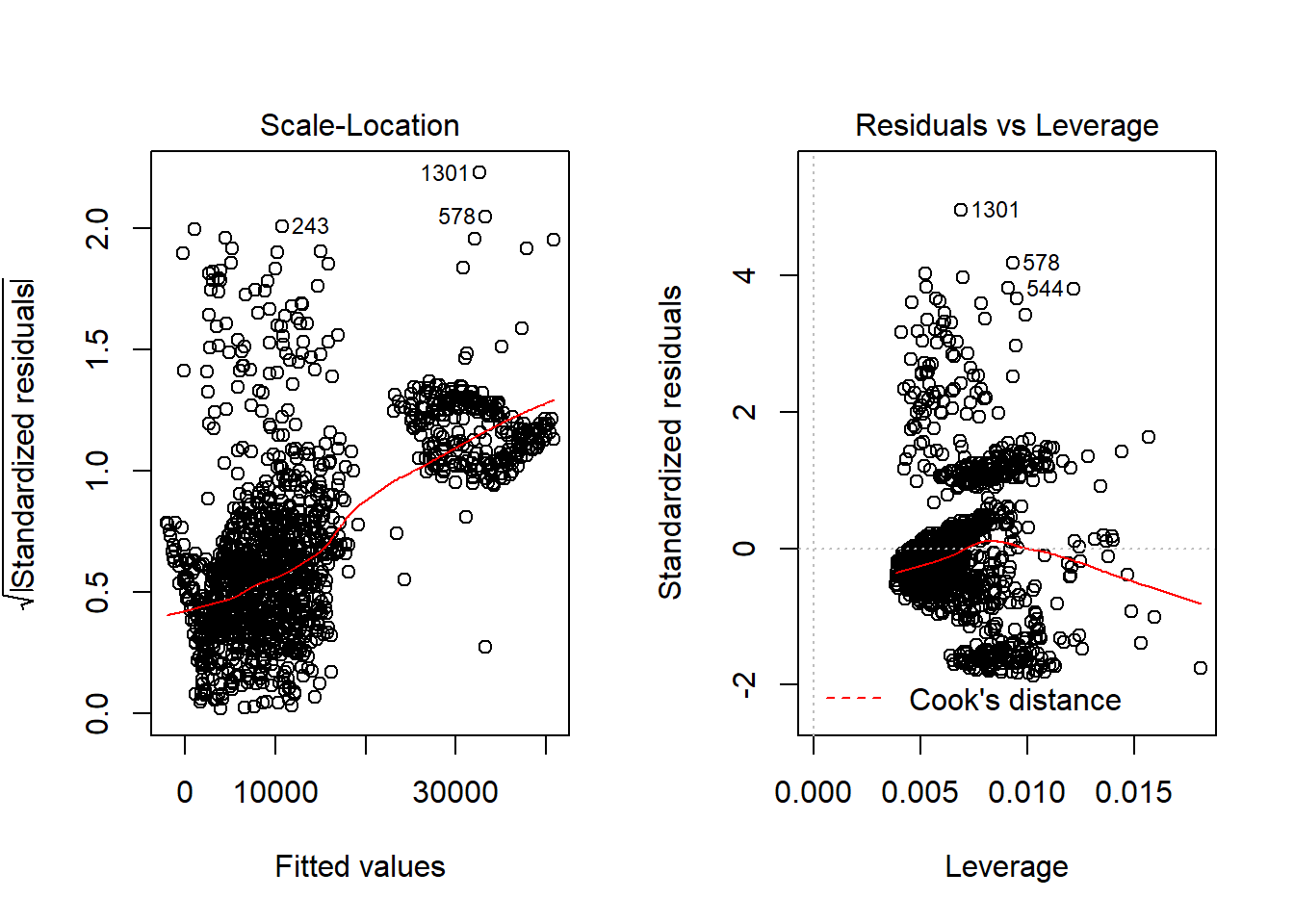
All in all, this model did quite well. Our outliers in the residuals is worrying however, not too surprising given the nature of the medical data.
26.4.2 Improving Model Performance
A key difference between the regression modeling and other machine learning approaches is that regression typically leaves feature selection and model specification to the user. Consequently, if we have subject matter knowledge about how a feature is related to the outcome, we can use this information to inform the model specification and potentially improve the model’s performance.
In linear regression, the relationship between an independent variable and the dependent variable is assumed to be linear, yet this may not necessarily be true. For example, the effect of age on medical expenditure may not be constant throughout all the age values; the treatment may become disproportionately expensive for oldest populations. Lets test this theory by adding a square term to the age feature.
##
## Call:
## lm(formula = charges ~ ., data = insurance)
##
## Residuals:
##      Min       1Q   Median       3Q      Max
## -11665.1  -2855.8   -944.1   1295.9  30826.0
##
## Coefficients:
##                  Estimate Std. Error t value Pr(>|t|)
## (Intercept)     -6596.665   1689.444  -3.905 9.91e-05 ***
## age               -54.575     80.991  -0.674 0.500532
## sexmale          -138.428    331.197  -0.418 0.676043
## bmi               335.211     28.467  11.775  < 2e-16 ***
## children          642.024    143.617   4.470 8.47e-06 ***
## smokeryes       23859.745    410.988  58.055  < 2e-16 ***
## regionnorthwest  -367.812    473.783  -0.776 0.437692
## regionsoutheast -1031.503    476.172  -2.166 0.030470 *
## regionsouthwest  -957.546    475.417  -2.014 0.044198 *
## age2                3.927      1.010   3.887 0.000107 ***
## ---
## Signif. codes:  0 '***' 0.001 '**' 0.01 '*' 0.05 '.' 0.1 ' ' 1
##
## Residual standard error: 6030 on 1328 degrees of freedom
## Multiple R-squared:  0.7537, Adjusted R-squared:  0.752
## F-statistic: 451.6 on 9 and 1328 DF,  p-value: < 2.2e-16
26.4.3 Transformations - Converting a numeric variable to a binary indicator
Suppose we have a hunch that the effect of a feature is not cumulative, rather it has an effect only after a specific threshold has been reached. For instance, BMI may have zero impact on medical expenditures for individuals in the normal weight range, but it may be strongly related to higher costs for the obese (that is, BMI of 30 or above). We can model this relationship by creating a binary obesity indicator variable that is 1 if the BMI is at least 30, and 0 if less. The estimated beta for this binary feature would then indicate the average net impact on medical expenses for individuals with BMI of 30 or above, relative to those with BMI less than 30.
To create this feature, we can use the ifelse() function, which for each element in a vector tests a specified condition and returns a value depending on wheather the condition is true or false.
insurance$bmi30 <- ifelse(insurance$bmi >= 30, 1, 0)

model <- lm(charges ~., data = insurance)

summary(model)
##
## Call:
## lm(formula = charges ~ ., data = insurance)
##
## Residuals:
## Min 1Q Median 3Q Max
## -12494.2 -3362.2 137.6 1312.0 29321.2
##
## Coefficients:
## Estimate Std. Error t value Pr(>|t|)
## (Intercept) -2943.176 1828.115 -1.610 0.107646
## age -28.533 80.445 -0.355 0.722875
## sexmale -166.295 328.315 -0.507 0.612584
## bmi 153.905 46.056 3.342 0.000856 ***
## children 630.402 142.366 4.428 1.03e-05 ***
## smokeryes 23857.543 407.353 58.567 < 2e-16 ***
## regionnorthwest -400.518 469.638 -0.853 0.393911
## regionsoutheast -888.533 472.833 -1.879 0.060440 .
## regionsouthwest -947.681 471.216 -2.011 0.044513 *
## age2 3.603 1.004 3.590 0.000342 ***
## bmi30 2727.552 547.618 4.981 7.17e-07 ***
## ---
## Signif. codes: 0 '***' 0.001 '**' 0.01 '*' 0.05 '.' 0.1 ' ' 1
##
## Residual standard error: 5977 on 1327 degrees of freedom
## Multiple R-squared: 0.7582, Adjusted R-squared: 0.7564
## F-statistic: 416.2 on 10 and 1327 DF, p-value: < 2.2e-1626.4.4 Model Specification: Adding interaction effects
Model specification – adding interaction effects So far, we have only considered each feature’s individual contribution to the outcome. What if certain features have a combined impact on the dependent variable? For instance, smoking and obesity may have harmful effects separately, but it is reasonable to assume that their combined effect may be worse than the sum of each one alone.
When two variables have a combined affect, this is known as an interaction. If we suspect that two variables interact, we can test this hypothesis by adding their interaction to the model. We do this by adding var1*var2 to the model. This includes the variables individually also, to determine whether there really is an interaction.
model <- lm(charges ~ age + children + sex + region + bmi30*smoker, data = insurance)
summary(model)
##
## Call:
## lm(formula = charges ~ age + children + sex + region + bmi30 *
## smoker, data = insurance)
##
## Residuals:
## Min 1Q Median 3Q Max
## -18829.3 -1872.4 -1306.7 -582.2 24710.6
##
## Coefficients:
## Estimate Std. Error t value Pr(>|t|)
## (Intercept) -1954.749 468.687 -4.171 3.23e-05 ***
## age 265.486 8.812 30.126 < 2e-16 ***
## children 524.041 102.338 5.121 3.49e-07 ***
## sexmale -479.924 247.474 -1.939 0.05268 .
## regionnorthwest -278.942 353.726 -0.789 0.43050
## regionsoutheast -587.138 348.845 -1.683 0.09259 .
## regionsouthwest -1160.701 354.505 -3.274 0.00109 **
## bmi30 201.748 281.354 0.717 0.47346
## smokeryes 13360.059 445.408 29.995 < 2e-16 ***
## bmi30:smokeryes 19856.483 612.121 32.439 < 2e-16 ***
## ---
## Signif. codes: 0 '***' 0.001 '**' 0.01 '*' 0.05 '.' 0.1 ' ' 1
##
## Residual standard error: 4502 on 1328 degrees of freedom
## Multiple R-squared: 0.8627, Adjusted R-squared: 0.8618
## F-statistic: 927.4 on 9 and 1328 DF, p-value: < 2.2e-1626.5 Putting it all Together: An Impoved Regression Model
To imporve our model performance, we had added:
- An interaction term for both
bmi30andsmoker. - A square term for age.
- An indicator for obesity.
We’ll train the model again using the lm() function, but this time we’ll add the newly constructed variables and the interaction term:
model2 <- lm(charges ~ age + age2 + bmi + bmi30 + children + sex + smoker +  bmi30*smoker + region, data = insurance)

summary(model2)
##
## Call:
## lm(formula = charges ~ age + age2 + bmi + bmi30 + children +
## sex + smoker + bmi30 * smoker + region, data = insurance)
##
## Residuals:
## Min 1Q Median 3Q Max
## -17296.4 -1656.0 -1263.3 -722.1 24160.2
##
## Coefficients:
## Estimate Std. Error t value Pr(>|t|)
## (Intercept) 134.2509 1362.7511 0.099 0.921539
## age -32.6851 59.8242 -0.546 0.584915
## age2 3.7316 0.7463 5.000 6.50e-07 ***
## bmi 120.0196 34.2660 3.503 0.000476 ***
## bmi30 -1000.1403 422.8402 -2.365 0.018159 *
## children 678.5612 105.8831 6.409 2.04e-10 ***
## sexmale -496.8245 244.3659 -2.033 0.042240 *
## smokeryes 13404.6866 439.9491 30.469 < 2e-16 ***
## regionnorthwest -279.2038 349.2746 -0.799 0.424212
## regionsoutheast -828.5467 351.6352 -2.356 0.018604 *
## regionsouthwest -1222.6437 350.5285 -3.488 0.000503 ***
## bmi30:smokeryes 19810.7533 604.6567 32.764 < 2e-16 ***
## ---
## Signif. codes: 0 '***' 0.001 '**' 0.01 '*' 0.05 '.' 0.1 ' ' 1
##
## Residual standard error: 4445 on 1326 degrees of freedom
## Multiple R-squared: 0.8664, Adjusted R-squared: 0.8653
## F-statistic: 781.7 on 11 and 1326 DF, p-value: < 2.2e-16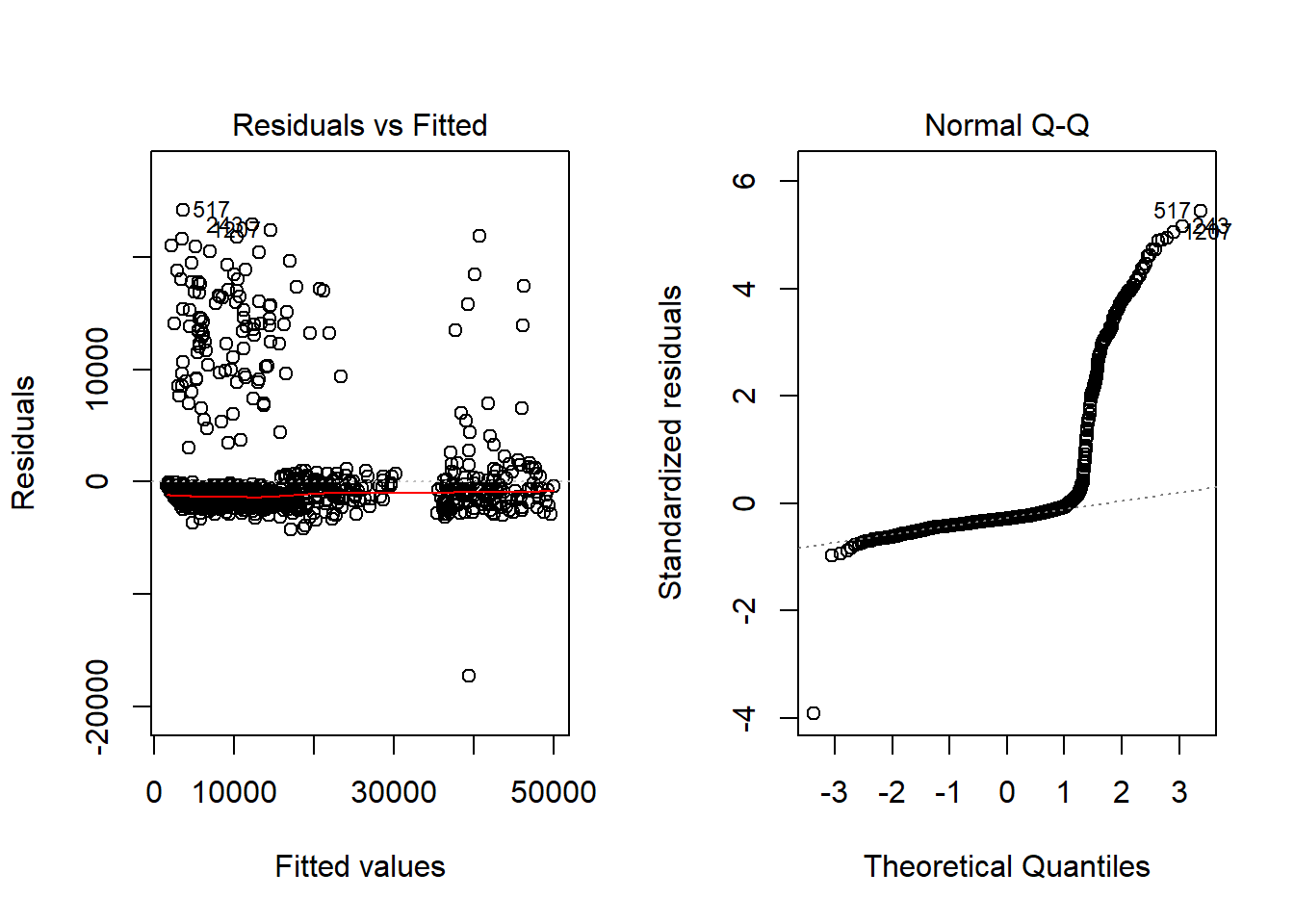
From the output above, it can be seen that we have increased model performance from 75% to 87% by adding these additional varibles.