14 Resampling

Resampling based procedures are ways to perform population based statistical inferences, while living within our data. Data Scientists tend to really like resampling based inferences, since they are very data centric procedures, they scale well to large studies and they often make very few assumptions.

14.1 The Bootstrap

The bootstrap is a tremendously useful tool for constructing confidence intervals and calculating standard errors for difficult statistics.

• For example, how would one derive a confidence interval for the median?

14.2 Example

Consider a datset:

# Load packages and data
library(UsingR)
data(father.son)

# Set variables
x <- father.son$sheight
n <- length(x)
B <- 10000

# Create and apply resamples
resamples <- matrix(sample(x , n * B, replace = TRUE), B, n)
resampledMedians <- apply(resamples, 1, median)

# Plot of distribution of resampled medians
ggplot(data = as.data.frame(resampledMedians), aes(x = resampledMedians)) +
  geom_density(color = "black", fill =  "orange") +
  geom_vline(aes(xintercept=median(resampledMedians)),
            color="blue", size=1) +
  geom_vline(aes(xintercept=(median(resampledMedians)+sd(resampledMedians))),
             color="lightblue", size=1) +
  geom_vline(aes(xintercept=(median(resampledMedians)-sd(resampledMedians))),
             color="lightblue", size=1) +
  ggtitle("Density Plot of Resampled Median") +
  xlab("Value of Medians") +
  ylab("Density")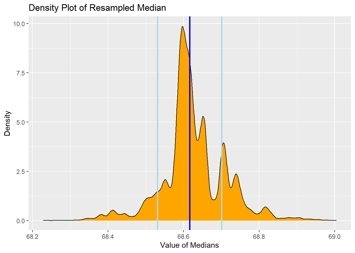

14.3 The Principle

• Suppose that there is a statistic that estimates some population parameter, but I don’t know its sampling distribution.
• The bootstrap principle suggests using the distribution defined by the data to approximate its sampling distribution
• In practice, the bootstrap principle is always carried out using simulation
  • The general procedure follows by first simulating complete data sets from the observed data with replacement
  • This is approximately drawing from the sampling distribution of that statistic, at least as far as the data is able to approximate the true population distribution

14.4 Nonparametric Bootstrap Algorithm Example

Boostrap procedure for calculating confidence intervals for the median from a dataset of \(n\) observations:

1. Sample \(n\) observations with replacement from the observed data resulting in one simulated complete dataset.
2. Take the median (or whatever statistic that you’re looking to estimate from the real distribution) of this simulated dataset.
3. Repeat the last two steps \(B\) times until you have \(B\) simulated medians. We want \(B\) to be large, so that the montecarlo error is small. We do not want the factor of how long you run your simulation for, to effectively dictate your results. (\(B\) should be > 10,000)
4. These medians are approximately drawn from the sampling distribution of the median of \(n\) observations; therefore we can:

• Draw a density plot (or histogram) of them
• Calculate their standard deviation to estimate the standard error of the median
• Take the \(2.5^{th}\) and \(97^{th}\) percentiles as a confidence interval for the median, resulting in a confidence interval for the estimation

14.5 Example:

This uses the Father-Son height data from the previous example where \(x\) is the son’s heights, \(B\) is the number of bootstrap resamples and \(n\) is the number of observations (in this case, the length of \(x\))

# Set number of Bootstrap resamples
B <- 10000

# Create the bootstrap and store data ina  matrix
resamples <- matrix(sample(x, n* B, replace = TRUE), B, n)

# Calculate the median for each row of the matrix and store the 10,000 medians
medians <- apply(resamples, 1, median)

sd(medians)

## [1] 0.08348666

quantile(medians, c(0.025, 0.975))

##     2.5%    97.5% 
## 68.43733 68.81414

ggplot(data = as.data.frame(medians), aes(x = medians)) +
  geom_density(color = "black", fill =  "white") +
  geom_vline(aes(xintercept=median(medians)),
            color="blue", size=1) +
  geom_vline(aes(xintercept=(median(medians)+sd(medians))),
             color="lightblue", size=1) +
  geom_vline(aes(xintercept=(median(medians)-sd(medians))),
             color="lightblue", size=1) +
  ggtitle("Density Plot of Resampled Median") +
  xlab("Value of Medians") +
  ylab("Density")

ggplot(data = as.data.frame(medians), aes(x = medians)) +
  geom_histogram(color = "black", fill =  "lightblue", binwidth = 0.025)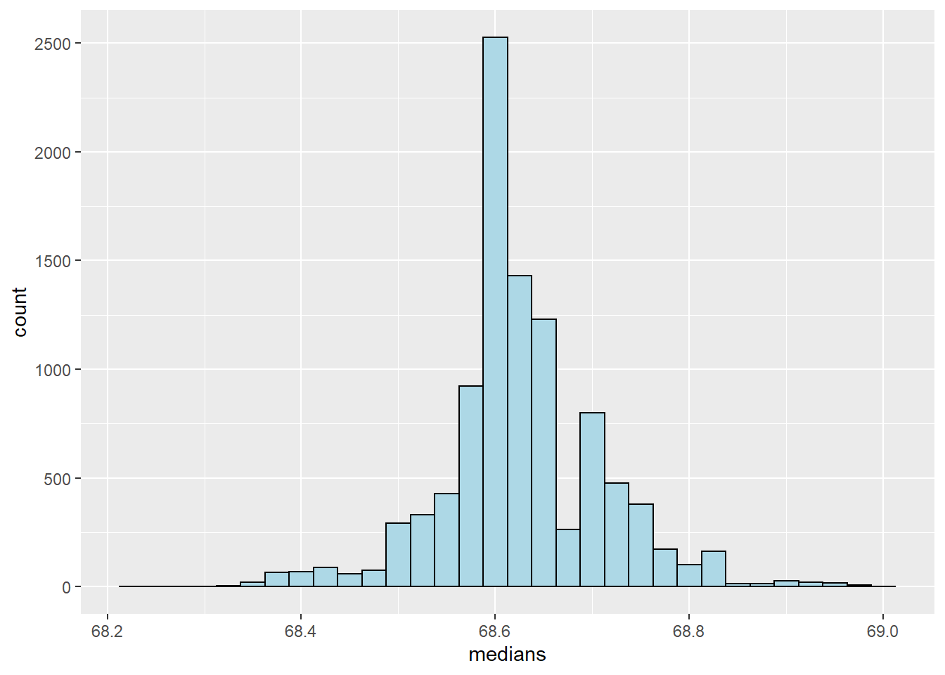

14.6 Notes

• The bootstrap is non-parametric
• Better percentile bootstrap confidence intervals correct for bias
• There are lots of variations on bootstrap procedures; the book “An introduction to the Bootstrap” by Efron and Tibshirani is a great place to start for information about the bootstrap and jackknife information