33 Exam 4:
Q1: Consider the space shuttle data ?shuttle in the MASS library. Consider modeling the use of the autolander as the outcome (variable name use). Fit a logistic regression model with autolander (variable auto) use (labeled as “auto” 1) versus not (0) as predicted by wind sign (variable wind). Give the estimated odds ratio for autolander use comparing head winds, labeled as “head” in the variable headwind (numerator) to tail winds (denominator).
data("shuttle")

library(dplyr)
library(MASS)

shuttle <- mutate(shuttle, use = relevel(use, ref="noauto"))
shuttle$use.bin <- as.integer(shuttle$use) - 1

mdl <- glm(use.bin ~ wind - 1, family = "binomial", data = shuttle)

summary(mdl)
##
## Call:
## glm(formula = use.bin ~ wind - 1, family = "binomial", data = shuttle)
##
## Deviance Residuals:
## Min 1Q Median 3Q Max
## -1.300 -1.286 1.060 1.073 1.073
##
## Coefficients:
## Estimate Std. Error z value Pr(>|z|)
## windhead 0.2513 0.1782 1.410 0.158
## windtail 0.2831 0.1786 1.586 0.113
##
## (Dispersion parameter for binomial family taken to be 1)
##
## Null deviance: 354.89 on 256 degrees of freedom
## Residual deviance: 350.35 on 254 degrees of freedom
## AIC: 354.35
##
## Number of Fisher Scoring iterations: 4## windhead windtail
## 1.285714 1.327273## [1] 0.96868880.969
Q2: Consider the previous problem. Give the estimated odds ratio for autolander use comparing head winds (numerator) to tail winds (denominator) adjusting for wind strength from the variable magn.
shuttle <- mutate(shuttle, use = relevel(use, ref="noauto"))
shuttle$use.bin <- as.integer(shuttle$use) - 1

mdl2 <- glm(use.bin ~ wind + magn - 1, family = "binomial", data = shuttle)

summary(mdl2)
##
## Call:
## glm(formula = use.bin ~ wind + magn - 1, family = "binomial",
## data = shuttle)
##
## Deviance Residuals:
## Min 1Q Median 3Q Max
## -1.349 -1.321 1.015 1.040 1.184
##
## Coefficients:
## Estimate Std. Error z value Pr(>|z|)
## windhead 3.635e-01 2.841e-01 1.280 0.201
## windtail 3.955e-01 2.844e-01 1.391 0.164
## magnMedium -1.010e-15 3.599e-01 0.000 1.000
## magnOut -3.795e-01 3.568e-01 -1.064 0.287
## magnStrong -6.441e-02 3.590e-01 -0.179 0.858
##
## (Dispersion parameter for binomial family taken to be 1)
##
## Null deviance: 354.89 on 256 degrees of freedom
## Residual deviance: 348.78 on 251 degrees of freedom
## AIC: 358.78
##
## Number of Fisher Scoring iterations: 4## windhead windtail magnMedium magnOut magnStrong
## 1.4383682 1.4851533 1.0000000 0.6841941 0.9376181## [1] 0.9684981The odds ratio is 0.968, meaning that when accounting for the magnitude of the wind velocity, it has little or no effect on the probability of using the autolander
Q3: If you fit a logistic regression model to a binary variable, for example use of the autolander, then fit a logistic regression model for one minus the outcome (not using the autolander) what happens to the coefficients?
##           Estimate Std. Error  z value  Pr(>|z|)
## windhead 0.2513144  0.1781742 1.410499 0.1583925
## windtail 0.2831263 0.1785510 1.585689 0.1128099## Estimate Std. Error z value Pr(>|z|)
## windhead -0.2513144 0.1781742 -1.410499 0.1583925
## windtail -0.2831263 0.1785510 -1.585689 0.1128099The signs are reversed when you take 1 - the outcome.
Q4: Consider the insect spray data InsectSprays. Fit a Poisson model using spray as a factor level. Report the estimated relative rate comapring spray A (numerator) to spray B (denominator).
data("InsectSprays")

mdl4 <- glm(count ~ spray -1, family = "poisson", data = InsectSprays)

summary(mdl4)$coef
## Estimate Std. Error z value Pr(>|z|)
## sprayA 2.6741486 0.07580980 35.274443 1.448048e-272
## sprayB 2.7300291 0.07372098 37.031917 3.510670e-300
## sprayC 0.7339692 0.19999987 3.669848 2.426946e-04
## sprayD 1.5926308 0.13018891 12.233229 2.065604e-34
## sprayE 1.2527630 0.15430335 8.118832 4.706917e-16
## sprayF 2.8134107 0.07071068 39.787636 0.000000e+00## sprayA sprayB sprayC sprayD sprayE sprayF
## 14.500000 15.333333 2.083333 4.916667 3.500000 16.666667## [1] 0.9456522So the relaive spray rate between Spray A and Spray B is 0.946
Q5: Consider a Poisson glm with an offset, t. So, for example, a model of the form glm(count ~ x + offset(t), family = poisson) where x is a factor variable comparing a treatment (1) to a control (0) and t is the natural log of a monitoring time. What is impact of the coefficient for x if we fit the model glm(count ~ x + offset(t2), family = poisson) where 2 <- log(10) + t? In other words, what happens to the coefficients if we change the units of the offset variable. (Note, adding log(10) on the log scale is multiplying by 10 on the original scale.)
mdl5.1 <- glm(count ~ spray, offset = log(count+1), family = poisson, data = InsectSprays)

mdl5.2 <- glm(count ~ spray, offset = log(count+1)+log(10), family = poisson, data = InsectSprays)

summary(mdl5.1)
##
## Call:
## glm(formula = count ~ spray, family = poisson, data = InsectSprays,
## offset = log(count + 1))
##
## Deviance Residuals:
## Min 1Q Median 3Q Max
## -1.16248 -0.09093 -0.01903 0.06738 0.65571
##
## Coefficients:
## Estimate Std. Error z value Pr(>|z|)
## (Intercept) -0.066691 0.075810 -0.880 0.379
## sprayB 0.003512 0.105745 0.033 0.974
## sprayC -0.325351 0.213886 -1.521 0.128
## sprayD -0.118451 0.150653 -0.786 0.432
## sprayE -0.184623 0.171920 -1.074 0.283
## sprayF 0.008422 0.103668 0.081 0.935
##
## (Dispersion parameter for poisson family taken to be 1)
##
## Null deviance: 9.5211 on 71 degrees of freedom
## Residual deviance: 4.9323 on 66 degrees of freedom
## AIC: 283.19
##
## Number of Fisher Scoring iterations: 4##
## Call:
## glm(formula = count ~ spray, family = poisson, data = InsectSprays,
## offset = log(count + 1) + log(10))
##
## Deviance Residuals:
## Min 1Q Median 3Q Max
## -1.16248 -0.09093 -0.01903 0.06738 0.65571
##
## Coefficients:
## Estimate Std. Error z value Pr(>|z|)
## (Intercept) -2.369276 0.075810 -31.253 <2e-16 ***
## sprayB 0.003512 0.105745 0.033 0.974
## sprayC -0.325351 0.213886 -1.521 0.128
## sprayD -0.118451 0.150653 -0.786 0.432
## sprayE -0.184623 0.171920 -1.074 0.283
## sprayF 0.008422 0.103668 0.081 0.935
## ---
## Signif. codes: 0 '***' 0.001 '**' 0.01 '*' 0.05 '.' 0.1 ' ' 1
##
## (Dispersion parameter for poisson family taken to be 1)
##
## Null deviance: 9.5211 on 71 degrees of freedom
## Residual deviance: 4.9323 on 66 degrees of freedom
## AIC: 283.19
##
## Number of Fisher Scoring iterations: 4## (Intercept) sprayB sprayC sprayD sprayE sprayF
## [1,] -0.06669137 0.003512473 -0.3253507 -0.1184511 -0.1846231 0.008422466
## [2,] -2.36927647 0.003512473 -0.3253507 -0.1184511 -0.1846231 0.008422466Turns out, the intercept changes but the coefficients stay exactly the same.
Q6: Consider the data: Using a knot point at 0, fit a linear model that looks like a hockey stick with two lines meeting at x=0. Include an intercept term, x and the knot point term. What is the estimated slope of the line after 0?
x <- -5:5
y <- c(5.12, 3.93, 2.67, 1.87, 0.52, 0.08, 0.93, 2.05, 2.54, 3.87, 4.97)

plot(x,y)

knots <- 0

splineTerms <- sapply(knots, function(knot) (x > knot)*(x - knot))

xmat <- cbind(1, x, splineTerms)

mdl6 <- lm(y~xmat-1)

yhat <- predict(mdl6)

lines(x, yhat, col = "red", lwd = 2)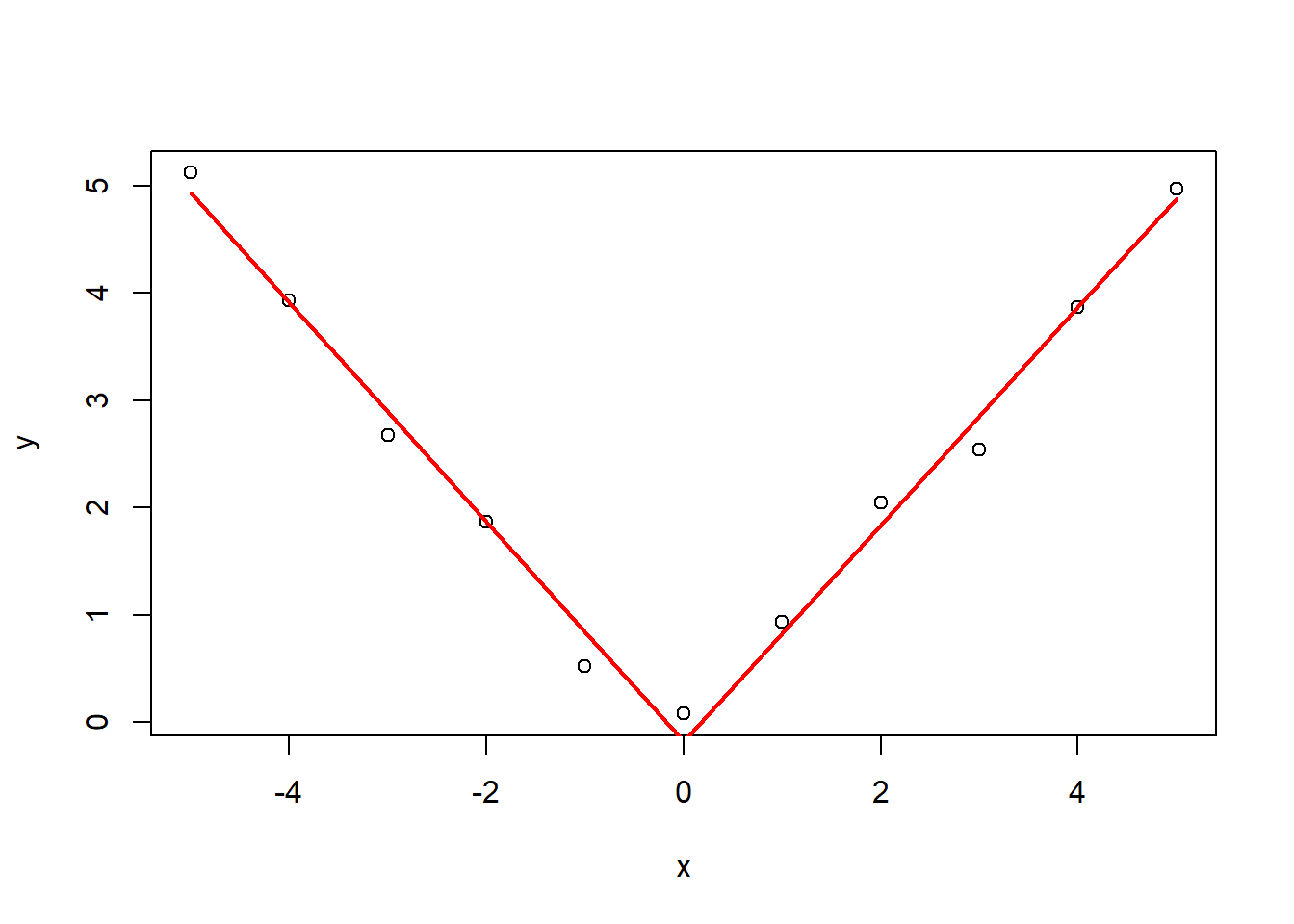
##
## Call:
## lm(formula = y ~ xmat - 1)
##
## Residuals:
##      Min       1Q   Median       3Q      Max
## -0.32158 -0.10979  0.01595  0.14065  0.26258
##
## Coefficients:
##       Estimate Std. Error t value Pr(>|t|)
## xmat  -0.18258    0.13558  -1.347    0.215
## xmatx -1.02416    0.04805 -21.313 2.47e-08 ***
## xmat   2.03723    0.08575  23.759 1.05e-08 ***
## ---
## Signif. codes:  0 '***' 0.001 '**' 0.01 '*' 0.05 '.' 0.1 ' ' 1
##
## Residual standard error: 0.2276 on 8 degrees of freedom
## Multiple R-squared:  0.996,  Adjusted R-squared:  0.9945
## F-statistic: 665 on 3 and 8 DF, p-value: 6.253e-10## [1] 1.013067The slope on the line after 0 is 1.01