7 Confidence Intervals

What is the likelihood that our interval contains \(\mu\)?

\(\bar{X_i}\) is approximately normal with mean \(\mu\) and SD \(\frac{\sigma}{\sqrt{n}}\)

Probability that \(\bar{X_i}\) is bigger than \(\mu + \frac{2 \sigma}{\sqrt{n}}\) or smaller than \(\mu + \frac{2 \sigma}{\sqrt{n}}\) is \(5 \%\).

\(\bar{X_i} \pm + \frac{2 \sigma}{\sqrt{n}}\) is called the \(95 \%\) interval for \(\mu\).

7.1 Example: Give CI for the average Son’s height

library(UsingR)

data(father.son)

x <- father.son$sheight

(mean(x) + c(-1, 1) * qnorm(0.975) * sd(x)/sqrt(length(x)))/12

## [1] 5.709670 5.737674

7.2 Sample Proportions

In the event that each \(X_i\) is 0 or 1 with common success probability \(p\) then \(\sigma^2= p(1-p)\)
The interval takes the form:

\[\hat{p} \pm z_{1-\frac{a}{2}} \sqrt{\frac{p(1-p)}{n}}\]

Replacing \(p\) by \(\hat{p}\) in the standard error results in what is called a Wald confidence interval for \(p\)
95% intervals, the following is a quick estimate for \(p\)

\[\hat{p} \pm \frac{1}{\sqrt{n}}\]

7.2.1 Example

Your campaign advisory says that in a random sample of 100 likely voters, 5 said that they would vote for you

Can you relax? Do you have this race in the bag?
Without access to a computer or calculator, how precise is this estimate?

\[\frac{1}{\sqrt{100} = 0.1}\] So a back of the envelope calculation gives an approximate interval between (0.46, 0.66), so we can’t rule out a result below 51% with 95% confidence.

This is not high enough for us to relax!

Rough guidelines, 100 for 1 decimal place, 10,000 for 2 decimal places, 1,000,000 for 3 decimal places.

round(1/sqrt(10^(1:6)), 3)

## [1] 0.316 0.100 0.032 0.010 0.003 0.001

7.3 Binomial Interval

0.56 + c(-1, 1) * qnorm(0.975) * sqrt(0.56 * 0.44/100)

## [1] 0.4627099 0.6572901

binom.test(56, 100)$conf.int

## [1] 0.4571875 0.6591640
## attr(,"conf.level")
## [1] 0.95

set.seed(1)

n <- 20
pvals <- seq(0.1, 0.9, by = 0.05)
nosim <- 1000

coverage <- sapply(pvals, function(p){
  phats <- rbinom(nosim, prob = p, size = n)/n
  ll <- phats - qnorm(0.975) * sqrt(phats * (1 - phats)/n)
  ul <- phats + qnorm(0.975) * sqrt(phats * (1 - phats)/n)
  mean(ll < p & ul > p)
})

qplot(pvals, coverage) +
  geom_line() + 
  geom_smooth(method = "loses") +
  geom_abline(intercept = 0.95, slope = 0, col = "red")

## `geom_smooth()` using formula 'y ~ x'

## Warning: Computation failed in `stat_smooth()`:
## object 'loses' of mode 'function' was not found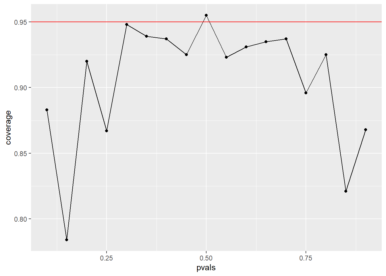

7.3.1 Small \(n\) Values

\(n\) isn’t large enough for the CLT to be applicable for many of the values of \(p\)
a quick fix for this, is to form the interval by adding two successes and two failures so that we gain the /Coll interval:

\[\frac{X+2}{n+4}\]

7.4 Poisson Interval

A nuclear pump fails 5 out of 94.32 days. Give a 95% confidence interval for the failure rate per day.

\(X \sim Poisson(X)\)
Estimate \(\hat{\lambda} - \frac{X}{t}\)
\(Var(\frac{\hat{\lambda}}{t})\)

# Number of obervations during period
x <- 5

# Observation period
t <- 94.32

# Estimate of the rate is x/t
lambda <- x/t

# CI estimate to 3dp is the rate estimate +- the standard normla quantile + std error 
round(lambda + c(-1,1) * qnorm(0.975) * sqrt(lambda/t), 3)

## [1] 0.007 0.099

# Or just use the test...
poisson.test(x, T = 94.32)$conf

## [1] 0.01721254 0.12371005
## attr(,"conf.level")
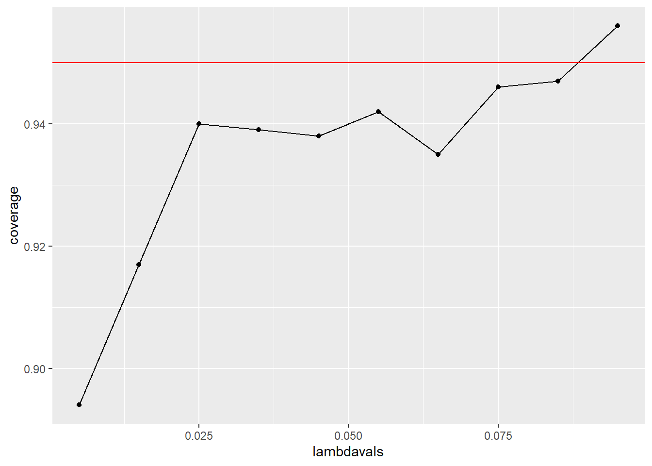
## [1] 0.95

7.5 Simulating Poisson Coverage

lambdavals <- seq(0.005, 0.1, by = 0.01)
nosim <- 1000
t <- 100

coverage <- sapply(lambdavals, function(lambda) {
  lhats <- rpois(nosim, lambda = lambda * t)/t
  ll <- lhats - qnorm(0.975) * sqrt(lhats/t)
  ul <- lhats + qnorm(0.975) * sqrt(lhats/t)
  mean(ll < lambda & ul > lambda)
  })

qplot(lambdavals, coverage) +
  geom_line() +
  geom_abline(slope = 0, intercept = 0.95, col = "red")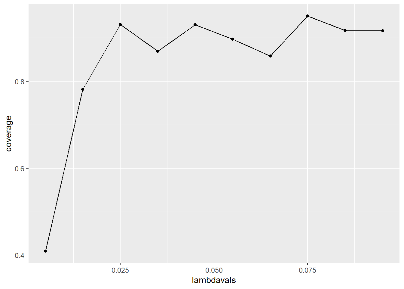

# What if we increase t -> 1000?
lambdavals <- seq(0.005, 0.1, by = 0.01)
nosim <- 1000
t <- 1000

coverage <- sapply(lambdavals, function(lambda) {
  lhats <- rpois(nosim, lambda = lambda * t)/t
  ll <- lhats - qnorm(0.975) * sqrt(lhats/t)
  ul <- lhats + qnorm(0.975) * sqrt(lhats/t)
  mean(ll < lambda & ul > lambda)
  })

qplot(lambdavals, coverage) +
  geom_line() +
  geom_abline(slope = 0, intercept = 0.95, col = "red")