21 Prediction

21.1 Prediction of Outcomes

Consider predicting \(Y\) as a value of \(X\)

• Predicting the price of a diamond given its mass

• Predicting the height of child given the heights of the parents

• The obvious estimate for prediction at point \(x_0\) is: \[\hat{\beta_0} + \hat{\beta_1} x_0\]

• A standard error is needed to create a prediction interval.

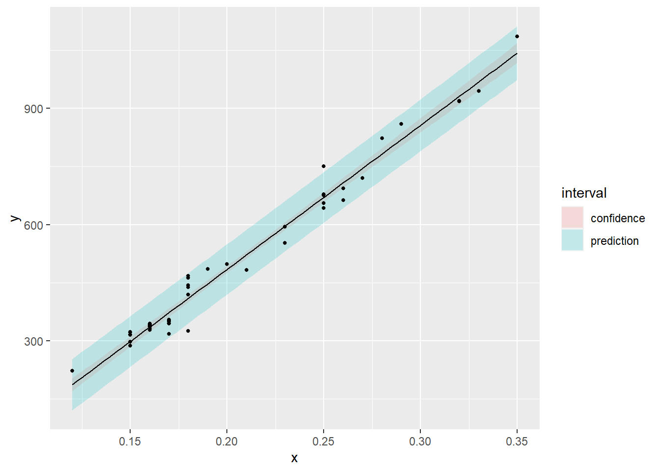
• There’s a distinction between intervals for the regression line at. \[x_0, \hat{\sigma} \sqrt{{1\over n}+{{(x_0 - \bar{X})^2}\over{\sum_{i=1}^n (X_i - \bar{X})^2}}}\]

• Prediction interval se at: \[x_0, \hat{\sigma} \sqrt{1+ {1\over n}+{{(x_0 - \bar{X})^2}\over{\sum_{i=1}^n (X_i - \bar{X})^2}}}\]

newx = data.frame(x = seq(min(x), max(x), length = 100))

p1 = data.frame(predict(fit, newdata = newx, interval = ("confidence")))
p2 = data.frame(predict(fit, newdata = newx, interval = ("prediction")))

p1$interval = "confidence"
p2$interval = "prediction"

p1$x = newx$x
p2$x = newx$x

dat = rbind(p1, p2)

names(dat)[1] = "y"

g <- ggplot(dat, aes(x = x, y = y)) +
  geom_ribbon(aes(ymin = lwr, ymax = upr, fill = interval), alpha = 0.2) +
  geom_line() +
  geom_point(data = data.frame(x = x, y = y), aes(x = x, y = y), size = 1)

g