54 Boosting

54.1 Basic Idea

Take lots of potentially weak predictors.
Weigh them and add them up.
Get a stronger predictor.

Start with a set of classifiers \(h_1, ..., h_k\)
- Examples: All possible trees, all possible regression models, all possible cut-offs.
Create a classifier that combines classification functions \[f(x) = sgn(\sum_{t=1}^T \alpha_t h_t(x))\]
- Goal is to minimise error (on training set)
- Iterative, select one \(h\) at each step
- Calculate weights based on errors
- Upweigh missed classifications and select \(h\)
- View Adaboost

54.2 Boosting in R

Boosting can be done with any subset of classifiers
One large subclass is gradient boosting
R has multiple boosting libraries. Differences include the choice of basic classification functions and combination rules.
- gbm - boosting with trees
- mboost - model based boosting
- ada - statistical boosting based on additive logistic regression
- gamBoost for boosting generalised additive models
Most of these are available in the caret package

54.3 Wage Example

library(gbm)
# Load Data
data(Wage)

# Subset and build training and testing sets
Wage <- subset(Wage, select = -c(logwage))

inTrain <- createDataPartition(y = Wage$wage ,
                               p = 0.7, list = FALSE)

training <- Wage[inTrain, ]
testing <- Wage[-inTrain, ]

# Model wage as a combination of all remaining variables
modFit <- train(wage ~ ., method = "gbm", 
                data = training, verbose = FALSE)

print(modFit)

## Stochastic Gradient Boosting 
## 
## 2102 samples
##    9 predictor
## 
## No pre-processing
## Resampling: Bootstrapped (25 reps) 
## Summary of sample sizes: 2102, 2102, 2102, 2102, 2102, 2102, ... 
## Resampling results across tuning parameters:
## 
##   interaction.depth  n.trees  RMSE      Rsquared   MAE     
##   1                   50      34.56805  0.3186570  23.32001
##   1                  100      34.03865  0.3286803  22.96212
##   1                  150      33.98890  0.3297850  22.98726
##   2                   50      33.98977  0.3315167  22.92748
##   2                  100      33.99139  0.3304338  23.01636
##   2                  150      34.09998  0.3274460  23.14241
##   3                   50      33.96126  0.3314366  22.95055
##   3                  100      34.15682  0.3258006  23.19512
##   3                  150      34.36910  0.3199571  23.40490
## 
## Tuning parameter 'shrinkage' was held constant at a value of 0.1
## 
## Tuning parameter 'n.minobsinnode' was held constant at a value of 10
## RMSE was used to select the optimal model using the smallest value.
## The final values used for the model were n.trees = 50, interaction.depth =
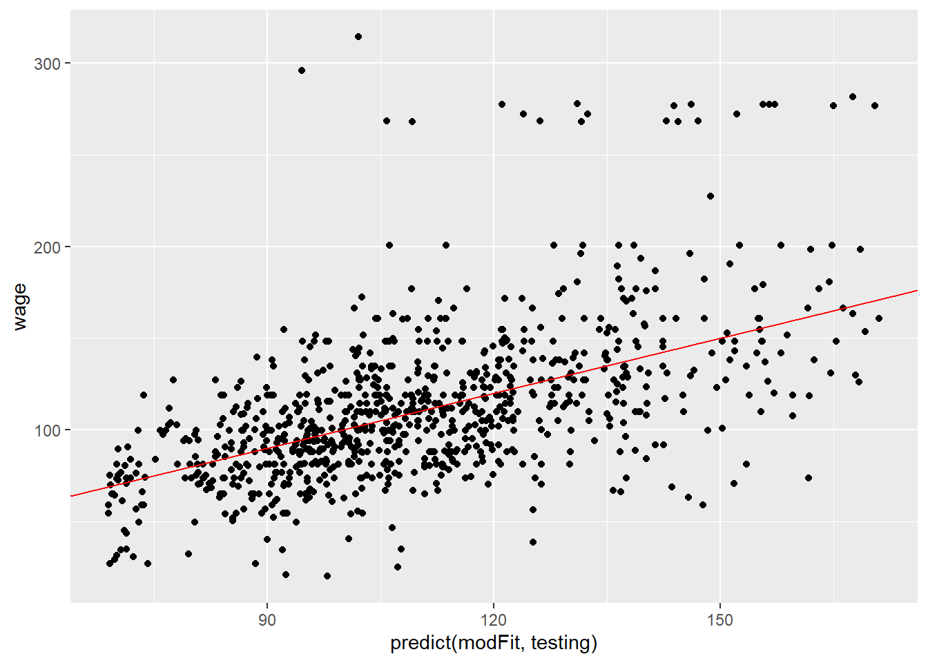
##  3, shrinkage = 0.1 and n.minobsinnode = 10.

# View the results
qplot(predict(modFit, testing), wage, data = testing) +
  geom_abline(slope = 1, col = "red")