27 Regression Trees and Model Trees
Trees for numeric prediction fall into two categories;
- Regression trees
- Model trees
Model trees are grown in much the same way as regression trees, but at each leaf, a multiple linear regression model is built from the examples reaching that node. Depending on the number of leaf nodes, a model tree may build tens or even hundreds of such models. This may make model trees more difficult to understand than the equivalent regression tree, with the benefit that they may result in a more accurate model.
Though traditional regression methods are typically the first choice for numeric prediction tasks, in some cases, numeric decision trees offer distinct advantages. For instance, decision trees may be better suited for tasks with many features or many complex, non-linear relationships among features and outcome. These situations present challenges for regression. Regression modeling also makes assumptions about how numeric data is distributed that are often violated in real-world data. This is not the case for trees.
One common splitting criterion is known as the standard deviation reduction \[SDR = sd(T) - \sum_i {{|T_i|}\over{T}} \times sd(T_i)\]
Where:
- \(sd(T)\) refers to the standard deviation in set \(T\).
- \(T_1, T_2, ... T_n\) are sets resulting from a split on a feature.
- \(|T|\) is the number of observations in set \(T\).
Essentially, the formula measures the reduction in standard deviation by comparing the standard deviation pre-split to the weighted standard deviation post-split.
27.1 Building the Model
redwine <- read.csv("wine.data", header=FALSE)
whitewine <- read.csv("whitewine.csv", header = TRUE)

whitewine$quality <- as.numeric(whitewine$quality)

# add some names to the features in the redwine data
name <- c("cultivar", "alcohol", "malic acid", "ash", "alcalinity of ash", "magnesium", "total phenols", "flavanoids", "nonflavanoid phenols", "proanthocyanins", "colour intensity", "hue", "od280/od315 of diluted wines", "proline")
names(redwine) <- name

str(whitewine)
## 'data.frame': 4899 obs. of 12 variables:
## $ fixedAcidity : num 7 6.3 8.1 7.2 7.2 8.1 6.2 7 6.3 8.1 ...
## $ volatileAcidity : num 0.27 0.3 0.28 0.23 0.23 0.28 0.32 0.27 0.3 0.22 ...
## $ citricAcid : num 0.36 0.34 0.4 0.32 0.32 0.4 0.16 0.36 0.34 0.43 ...
## $ residualSugar : num 20.7 1.6 6.9 8.5 8.5 6.9 7 20.7 1.6 1.5 ...
## $ chlorides : num 0.045 0.049 0.05 0.058 0.058 0.05 0.045 0.045 0.049 0.044 ...
## $ freeSulfurDioxide : num 45 14 30 47 47 30 30 45 14 28 ...
## $ totalSulfurDioxide: num 170 132 97 186 186 97 136 170 132 129 ...
## $ density : num 1.001 0.994 0.995 0.996 0.996 ...
## $ pH : num 3 3.3 3.26 3.19 3.19 3.26 3.18 3 3.3 3.22 ...
## $ sulphates : num 0.45 0.49 0.44 0.4 0.4 0.44 0.47 0.45 0.49 0.45 ...
## $ alcohol : num 8.8 9.5 10.1 9.9 9.9 10.1 9.6 8.8 9.5 11 ...
## $ quality : num 6 6 6 6 6 6 6 6 6 6 ...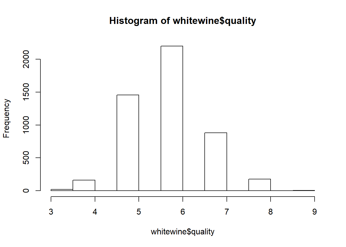
wine_train <- whitewine[1:3750, ]
wine_test <- whitewine[3751:4898, ]
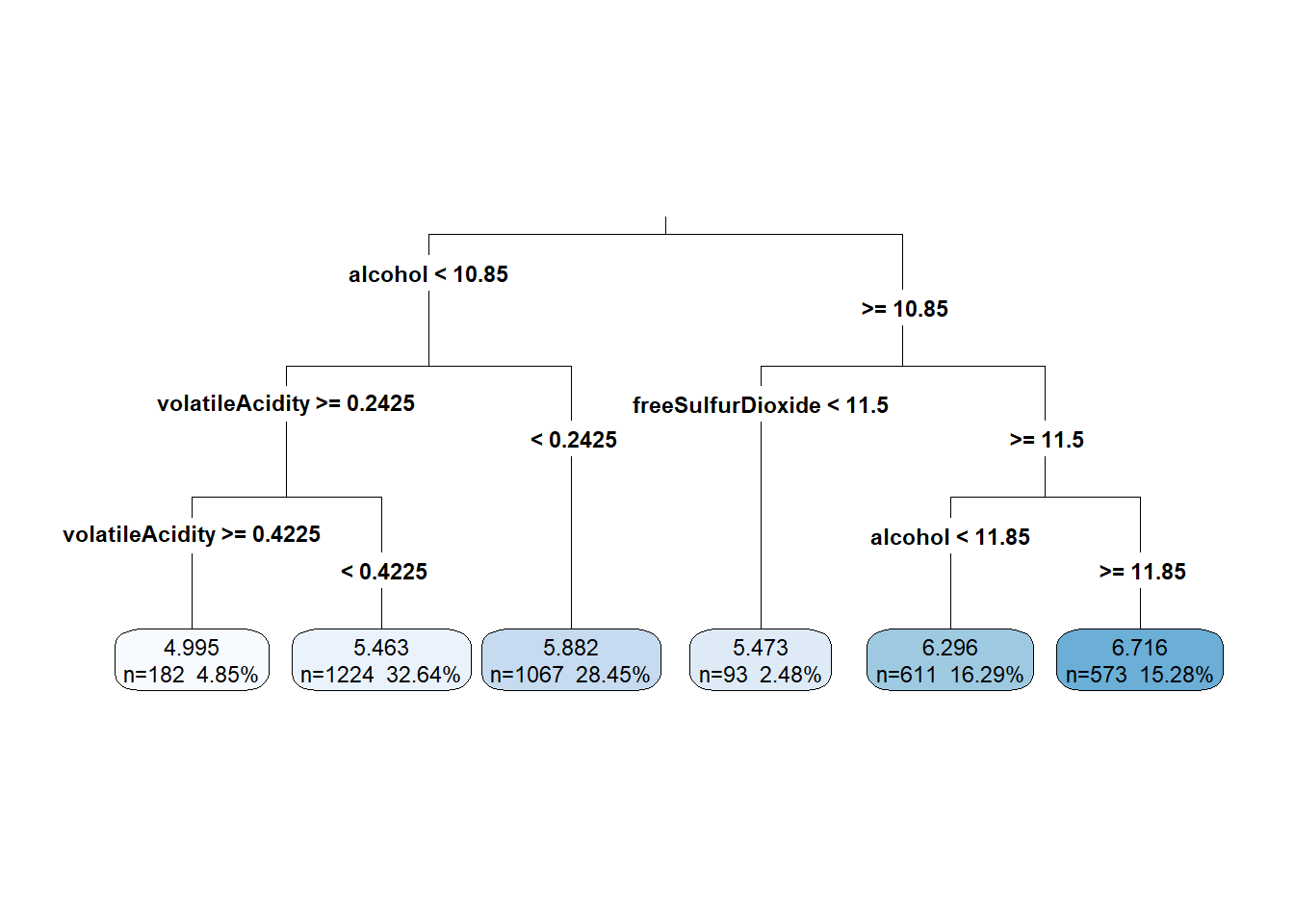
rp_model <- rpart(quality ~ ., data = wine_train)
rp_model## n= 3750
##
## node), split, n, deviance, yval
## * denotes terminal node
##
## 1) root 3750 3140.06000 5.886933
## 2) alcohol< 10.85 2473 1510.66200 5.609381
## 4) volatileAcidity>=0.2425 1406 740.15080 5.402560
## 8) volatileAcidity>=0.4225 182 92.99451 4.994505 *
## 9) volatileAcidity< 0.4225 1224 612.34560 5.463235 *
## 5) volatileAcidity< 0.2425 1067 631.12090 5.881912 *
## 3) alcohol>=10.85 1277 1069.95800 6.424432
## 6) freeSulfurDioxide< 11.5 93 99.18280 5.473118 *
## 7) freeSulfurDioxide>=11.5 1184 879.99920 6.499155
## 14) alcohol< 11.85 611 447.38130 6.296236 *
## 15) alcohol>=11.85 573 380.63180 6.715532 *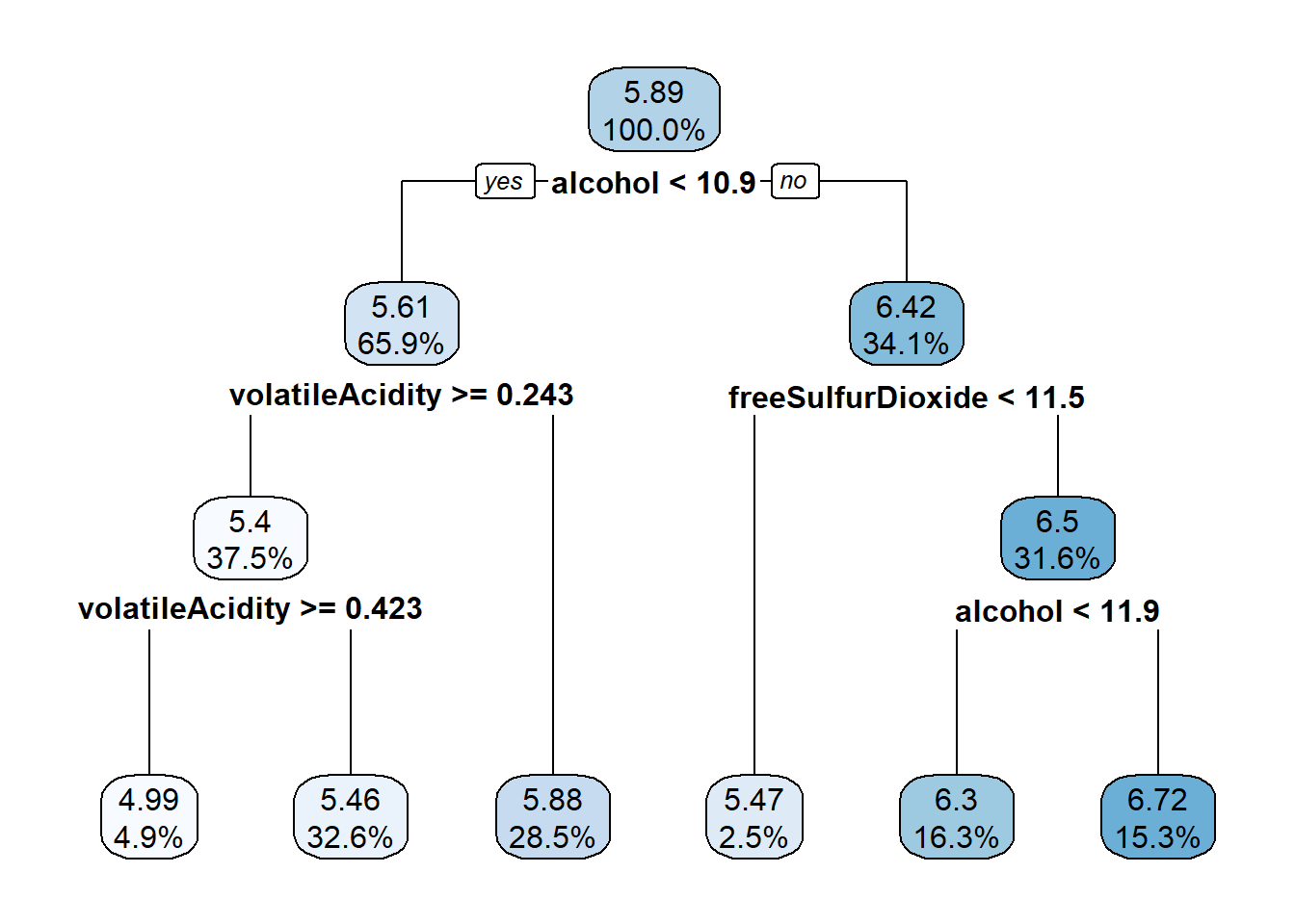
27.2 Evaluating the Model
##    Min. 1st Qu.  Median    Mean 3rd Qu.    Max.
## 4.995 5.463 5.882 5.999 6.296 6.716## Min. 1st Qu. Median Mean 3rd Qu. Max.
## 3.000 5.000 6.000 5.848 6.000 8.000