47 Covariate Creation
Garbage in \(\rightarrow\) Garbage out. For this reason it is important to know how to create the covariates (also called features or predictors) that are fed into a machine learning algorithm.
47.1 Two Levels of Covariate Creation
Level 1: From raw data to covariate:
- Depends heavily on the application
- The balancing act of summarisation vs information loss (compression ratio)
- Text files: frequency of words, frequency of phrases (ngrams), frequency of capital letters…
- Images: Edges, corners, blobs, ridges (Computer vision face detection)
- Webpages: Number and type of images, position of elements, colours, videos (A/B testing)
- People: Height, Weight, hair colour, sex, country of origin.
- The more knowledge of the system that you have, the better job you will do.
- When in doubt, err on the side of more features (Will always explain more variance, but be careful for confounding variables especially with linear models)
- This process can be automated but do so with caution (algorithmic bias can be a huge problem, especially when it is not possible to find sources of said bias)
Raw text file (for example a text or email) is transformed into a set of measurable (features) with some degree of compression. This could be a list of values such as:
- Number of ‘$’ signs
- Proportion of capital letters
- Number of times the word ‘you’ is used
Level 2: Transforming tidy covariates:
Sometimes you’ll want to create new covariates by transforming already existing covariates, for example a binary thresholding variable such as bmi could be used to create a logical covariate for weather a patient is obese or not bmi>25.
- More necessary for some methods such as regression models and support vector machines (as they’re heavily influenced by the distribution of the data) than for others such as regression trees (as these classification models do not need the data to look a certain way).
- Should be done only on the training set
- The best approach is though exploratory analysis
- New covariates should be added to data frames
The Basic idea in the following example is to convert factor variables into indicator variables. We will do this with the dummyVars() function from the caret package. This will effectively change variable from being qualitative to being quantitative.
# Load Data
library(ISLR); data(Wage);

# Create training and testing set
inTrain <- createDataPartition(y = Wage$wage,
                               p = 0.7, list = FALSE)
training <- Wage[inTrain, ]
testing <- Wage[-inTrain, ]

table(training$jobclass)
##
## 1. Industrial 2. Information
## 1090 1012# Lets convert the factor variables into indicator variables (Dummy Variables) using the 'dummyVars' function
dummies <- dummyVars(wage ~ jobclass, data= training)
head(predict(dummies, newdata = training))## jobclass.1. Industrial jobclass.2. Information
## 86582 0 1
## 161300 1 0
## 155159 0 1
## 11443 0 1
## 450601 1 0
## 377954 0 147.2 Removing Zero Covariates
Something else that can happen is that some variables can have no variability in them at all. Sometimes you’ll create a feature that says for example: For emails does it have any letters in them at all? In this case, it turns out that all emails have letters in them, so it’s a useless predictor that needs removing.
We will do this with the nearZeroVar() function from the caret package.
# Lets check how helpful all of our covariants are, using the measure of  'Near Zero Variance' using the 'nearZeroVar' function
nsv <- nearZeroVar(training, saveMetrics = TRUE)
nsv
## freqRatio percentUnique zeroVar nzv
## year 1.066465 0.33301618 FALSE FALSE
## age 1.080000 2.90199810 FALSE FALSE
## maritl 3.072495 0.23786870 FALSE FALSE
## race 8.641791 0.19029496 FALSE FALSE
## education 1.433610 0.23786870 FALSE FALSE
## region 0.000000 0.04757374 TRUE TRUE
## jobclass 1.077075 0.09514748 FALSE FALSE
## health 2.406807 0.09514748 FALSE FALSE
## health_ins 2.269051 0.09514748 FALSE FALSE
## logwage 1.011628 19.12464320 FALSE FALSE
## wage 1.011628 19.12464320 FALSE FALSE## freqRatio percentUnique zeroVar nzv
## region 0 0.04757374 TRUE TRUE47.3 Spline Basis
Linear regression and generalised linear models are great for fitting straight lines to your data, however, what if we want curved lines for whatever reason? This is where Splines fit in.
We can use the splines package to do this. We pass a continuous covariate such as training$age to the bs() function, which will create a polynomial, the number of degrees of freedom of which are decided by the df argument.
# Load 'splines' package that contains the 'bs' function
library(splines)

# Create our basis
bsBasis <- bs(training$age, df = 3)
head(bsBasis)
## 1 2 3
## [1,] 0.2368501 0.02537679 0.000906314
## [2,] 0.4163380 0.32117502 0.082587862
## [3,] 0.4308138 0.29109043 0.065560908
## [4,] 0.3625256 0.38669397 0.137491189
## [5,] 0.4241549 0.30633413 0.073747105
## [6,] 0.3776308 0.09063140 0.007250512# Fit a curve to a linear model
modelFit <- lm(wage ~ bsBasis, data = training)
plot(training$age, training$wage, pch = 19, cex = 0.5, xlab = "Age", ylab = "Wage", main = "Predicting Wage via Age using 3rd Degree Spline")
points(training$age, predict(modelFit, mdewdata = training), col = 'red', pch = 19, cex =0.5)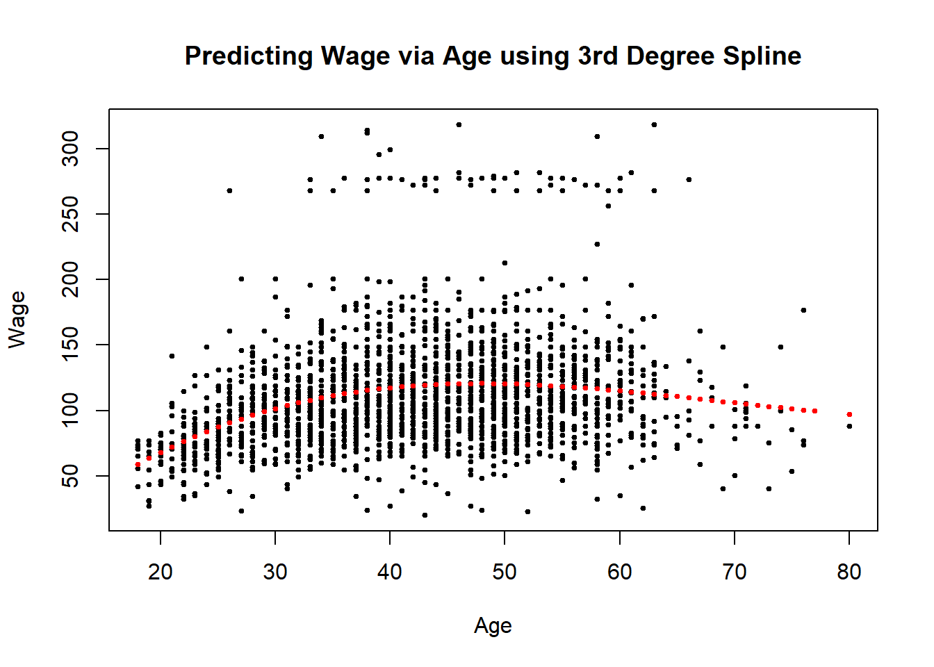
So then on the test set we’ll have to predict the same variables. This is the critical idea for machine learning when you create new covariates. You create the covariates on the testing data by using the exact same procedure as you did on the training data. We do this by using the predict function
47.4 Notes
For level 1:
- Science is key; Google “Feature extraction for [data type]”
- Err on the side of over creation of features to explain more variance
- In some application automated feature extraction may be necessary such as with images or with voices (Deep learning; CNN)