25 Residuals Diagnostics and Variation
Recall from before that the vertical distances between the observed data points and the fitted regression line are called residuals. We can generalize this idea to the vertical distances between the observed data and the fitted surface in multivariable settings.
- The linear model: \(Y_i = \sum_{k=1}^p X_{ik} \beta_j + \epsilon_i\)
- Assume here that: \(\epsilon_i = N(0, \sigma^2)\)
- Define the residuals as \(e_i = Y_i - \hat{Y_i} = Y_i = \sum_{k=1}^p X_{ik} \hat{\beta_j}\)
- Our estimate of the residual variation is \(\hat{\sigma}^2 = \frac{\sum_{i=1}^n e_i^2}{n-p}\)
25.0.1 Influential, High Leverage and Outlying Points
- Leverage: Leverage can be explained as how far away from the means of the Xs the data point sits.
- Influence: Influence explains weather or not a point chooses to use it’s leverage.
25.0.2 Summary of the plot
Outliers can be the result of real or spurious processes. Outliers can also conform to the regression relationship by lying close to the regression line, while existing far from the other data.
25.1 Influence Measures
?influence.measuresprovides a laundry list of measures of influence.rstudentandrstandardare attempts to standardise the residuals by dividing by an appropriate measure.hatvaluesis a measure of influence.- How do we measure actual influence instead of potential for influence ? You would have to take out the data point, refit the model and see if it made a positive difference and compare it to whatever aspect of the model you wish to improve.
dfbetaslooks a how much the slope coefficients change.dffitsprovides us with one dffit per data point. cooks.distancesummarises overall change in coefficients.
25.1.1 Case 1: Linear Trend when there should not be
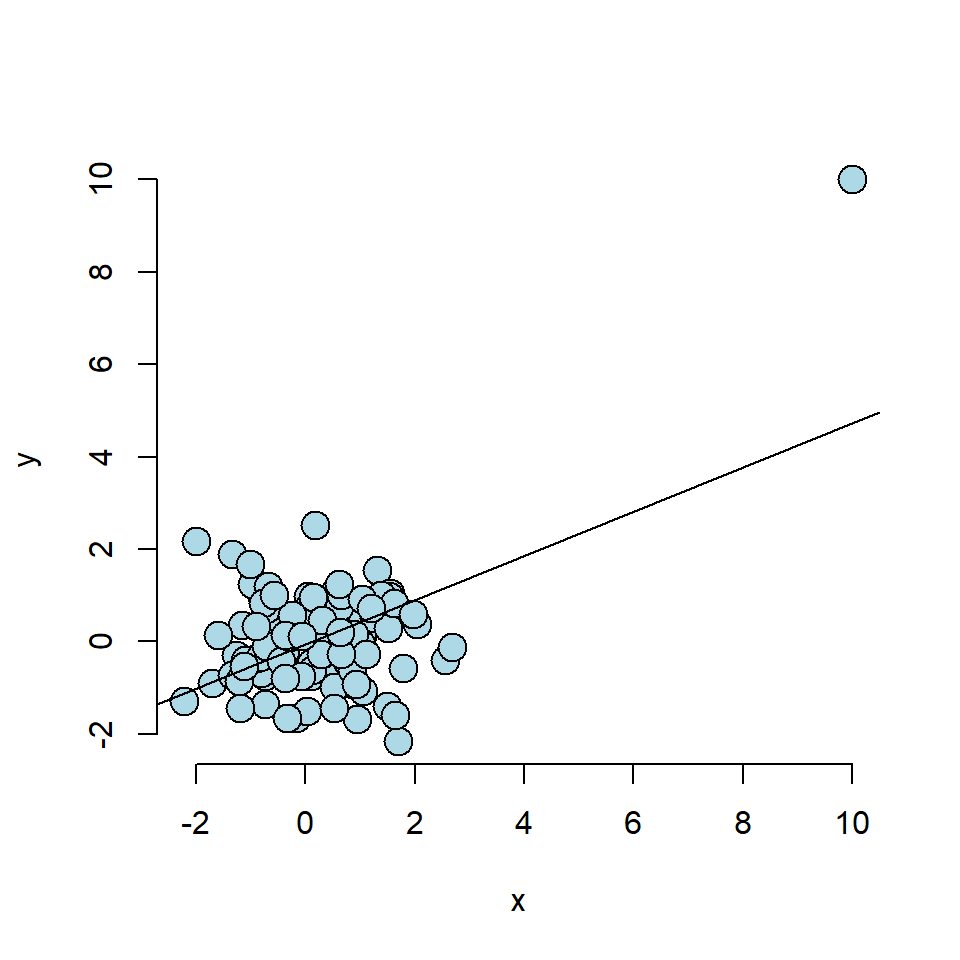
The point c(10,10) has created a stron regression relation where there should not be one.
Showing some of the diagnostic values:
##      1      2      3      4      5      6      7      8      9     10
## 7.889 0.060 -0.159 0.001 0.021 -0.034 -0.016 0.016 -0.003 0.042## 1 2 3 4 5 6 7 8 9 10
## 0.491 0.015 0.018 0.010 0.015 0.022 0.013 0.016 0.010 0.011We can see that the first point, is the outlier, where it has a dfbeta score, orders of magnitude above the others, so if we were looking for outliers, we would single this point out.
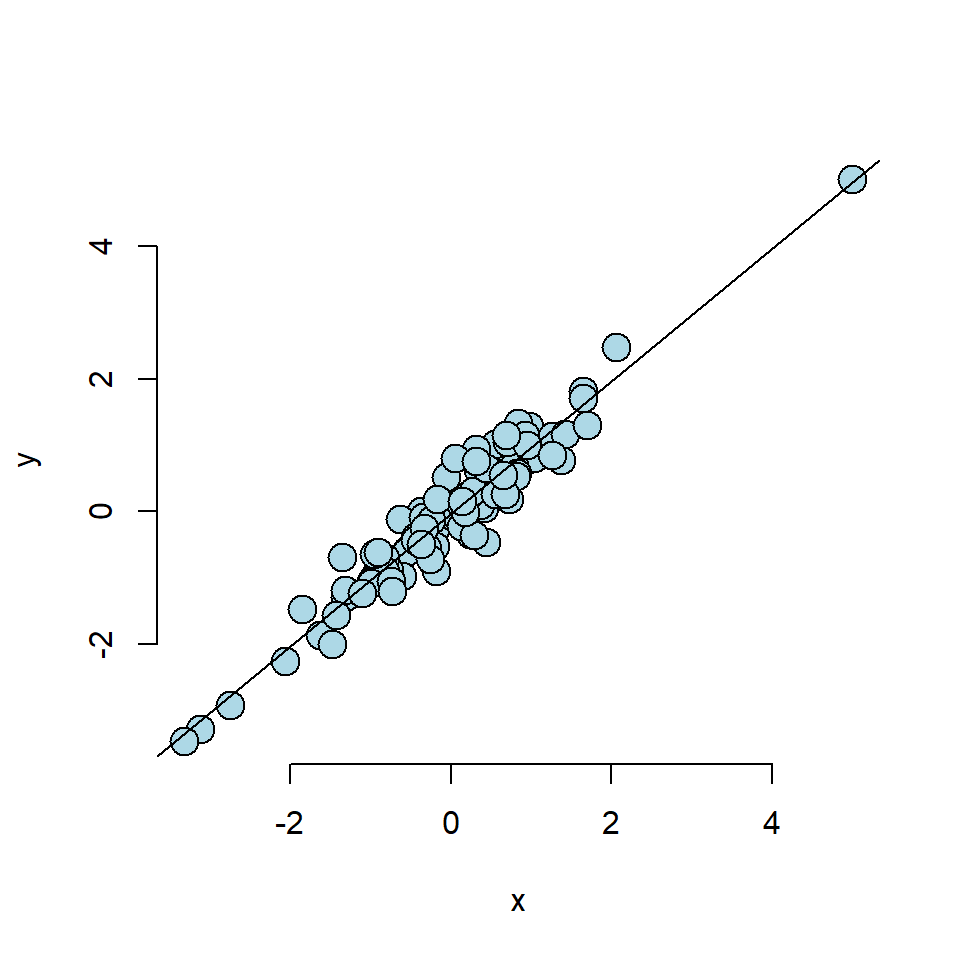
25.1.2 Case 2: Linear trend with outlier
##      1      2      3      4      5      6      7      8      9     10
##  0.076 -0.004  0.029 -0.027  0.102  0.095 -0.041 -0.047  0.001  0.002
## 1 2 3 4 5 6 7 8 9 10
## 0.215 0.010 0.015 0.025 0.032 0.032 0.017 0.011 0.010 0.013Looking at the dfbetas here, the first point seems large, but it is nowhere near as large as in case 1, so this does appear to have some influence still. However, when looking at the hatvalues, it has a much higher hatvalue than any of the other points as it is ouside of the range of the x values but it does adhere to the regression relationship.
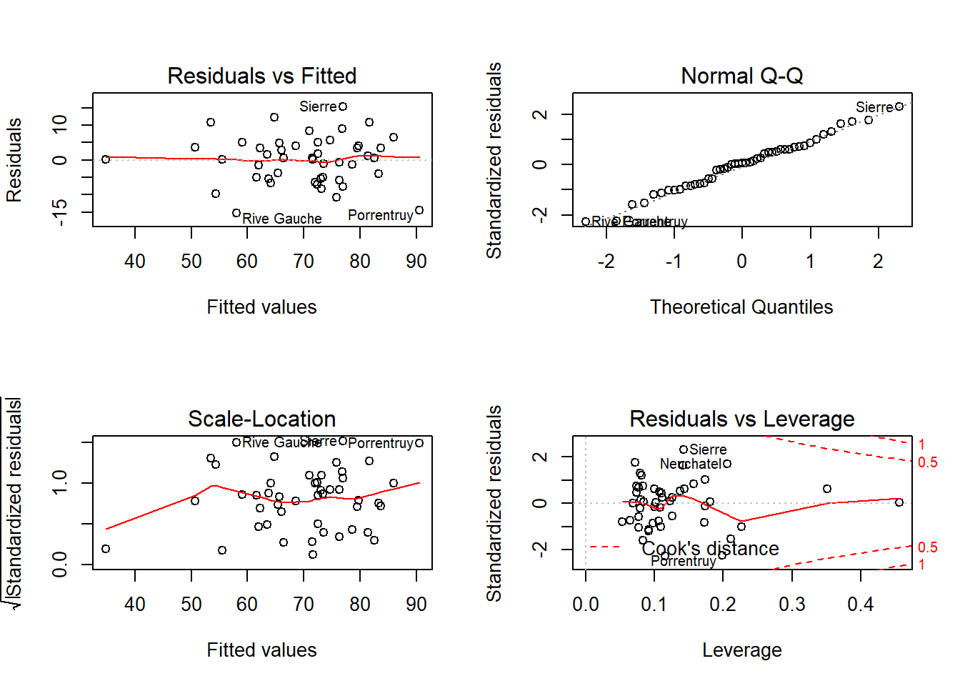
25.1.3 The Plot Summary
- Residuals vs Fitted plot tests for constant variance.
- Normal Q-Q plots are designed to test for residual normality.
- Scale-Location tests for standardised residuals (scaled to look like a T-satistic) plotted against the fitted values.
- Residuals vs leverage look at - well - leverage.