55 Model Based Prediction
55.1 Basic Idea
- Assume the data follow a probabilistic model
- Use Bayes’ theorem to identify optimal classifiers
Pros:
- Can take advantage of structure of the data
- May be computationally convenient
- Are reasonably accurate on real problems
Cons:
- Make additional assumptions about the data
- When the model is incorrect, you may get reduced accuracy
55.2 Model Based Approach
- Our goal is to build a parametric model for conditional distributions \(P(Y = k|X = x)\)
- A typical approach is to apply Bayes Theorem
\[Pr(Y = k|X = x) = \frac{Pr(X = x|Y = k)~Pr(Y = k)}{\sum_{l=1}^K ~ Pr(X = x|Y = l) ~ Pr(Y = l)}\] \[Pr(Y = k|X = x) = \frac{f_k(x)\pi_k}{\sum_{l=1}^K f_l(x)\pi_l}\] Where:
- \(f_k(x)\) represents the model for the \(x\) variables
- \(\pi_k\) represents the model for the prior probabilities
Where:
- \(Pr(Y = k|X = x)\) is the probability that \(Y = k\) given that \(X = x\)
- \(Y\) is the outcome
- \(k\) is the specific class given a particular set of predictor variables so that \(X\) is equal to the value of \(x\).
- Typically prior probabilities \(\pi_k\) are set in advance.
- A common choice for \(f_k(x)\) is a Gaussian distribution: \[f_k(x) = \frac{1}{\sigma_i \sqrt{2\pi}}e^{\frac{(x-\mu_k)^2}{\sigma_k^2}}\]
- Estimate the parameters \((\mu_k, \sigma_k^2)\) from the data.
- Once we have estimated these parameters, we can then classify the class as that with the highest value of \(P(Y = k|X = x)\)
55.3 Classifying Using the Model
A range of models use this approach:
- Linear discriminant analysis assumes \(f_k(x)\) is a multivariate Gaussian with same covariances.
- Quadratic discriminant analysis assumes \(f_k(x)\) is a multivariate Gaussian with different covariances
- Model Based Prediction assumes more complicated versions for the covariance matrix
- Naive Bayes assumes independence between features for model building
55.4 Why Linear Discriminant Analysis?
\[log \frac{Pr(Y = k|X = x)}{Pr(Y = j|X = x)}\] \[= log \frac{f_k(x)}{f_j(x)} + log \frac{\pi_k}{\pi_j}\] \[= log \frac{\pi_k}{\pi_j} - \frac{1}{2}(\mu_k + \mu_j)^T \sum^{-1}(\mu_k + \mu_j) + x^T \sum{-1}(\mu_k - \mu_j)\]
55.5 Decision Boundaries
Each ring below represents a different Gaussian distribution corresponding to a different class. The decision boundaries are created from the points of intersection between these Gaussian distributions.

55.6 Discriminant Function
\[\delta_k(x) = x^T \sum^{-1} \mu_k - \frac{1}{2} \mu_k \sum^{-1} \mu_k + log(\mu_k)\] Where:
\(\mu_k\) is the mean of the class \(k\) for all features
\(\sum^{-1}\) is the inverse of the covariance matrix
The observation is chosen by maximising the value of \(\delta_k(x)\)
Decide on class based on \(\hat{Y}(x) = argmax_k ~~\delta_k(x)\)
Usually estimate parameters with maximum likelihood.
55.7 Naive Bayes
Suppose we have many predictors, we would want to model: \(Pr(Y = k|X_1, ..., X_m)\)
We could use Bayes Theorem to get:
\[Pr(Y = k|X_1, ..., X_m) = \frac{\pi_k Pr(X_1, ..., X_m|Y = k)}{\sum_{l=1}^K Pr(X_1, ..., X_m|Y = k) \pi_l}\] \[\propto~~\pi_k Pr(X_1, ..., X_m|Y = k)\] This can be written:
\[P(X_1, ..., X_m|Y = k) = \pi_k P(X_1| Y =k) P(X_2, ..., X_m| X_1, Y = k)\] \[P\pi_k P(X_1| Y =k) P(X_2, ..., X_m| X_1, Y = k)P(X_3, ..., X_m|X_1, X_2, Y = k)\] \[\pi_k P(X_1| Y =k) P(X_2, ..., X_m| X_1, Y = k)...P(X_m|X_1, ..., X_{m-1}, Y = k)\] With assumptions, this simplifies to: \[\approx \pi_k P(X_1|Y = K)P(X_2|Y = K)...P(X_m|Y = K)\]
55.8 Example: Iris Data
##
##     setosa versicolor  virginica
##         50         50         50
# Create data partitions
inTrain <- createDataPartition(y = iris$Species,
p = 0.7, list = FALSE)
training <- iris[inTrain, ]
testing <- iris[-inTrain, ]
dim(training); dim(testing)## [1] 105 5## [1] 45 5# Create model using train function
modlda <- train(Species ~., data = training, method = "lda")
modnb <- train(Species ~., data = training, method = "nb")
# Predict with each model
plda <- predict(modlda, testing)
pnb <- predict(modnb, testing)
# View results
table(plda, pnb)## pnb
## plda setosa versicolor virginica
## setosa 15 0 0
## versicolor 0 14 0
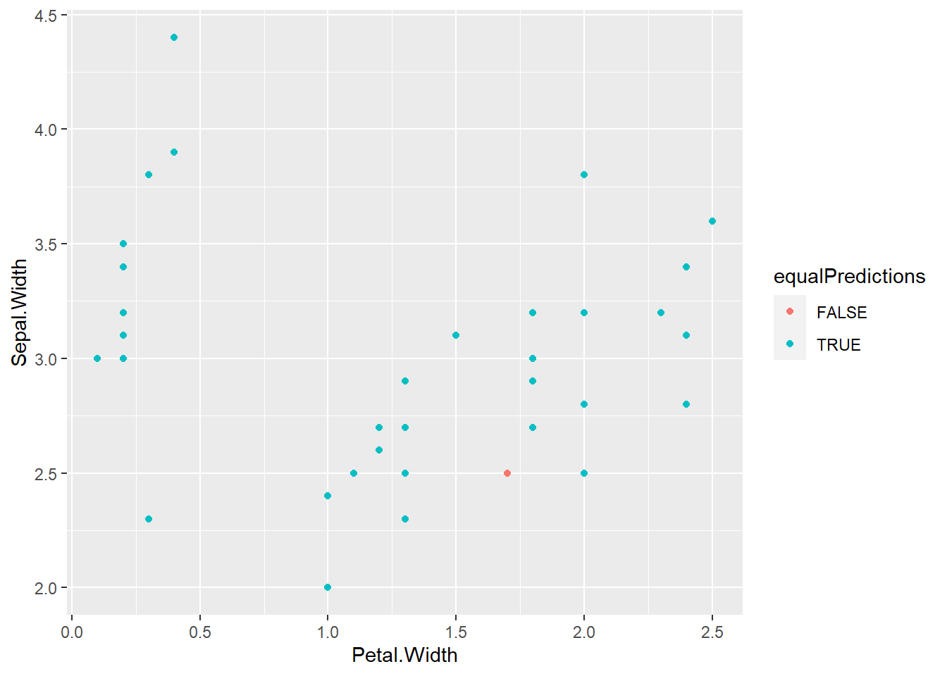
## virginica 0 1 15# View differences between results
equalPredictions <- (plda == pnb)
qplot(Petal.Width, Sepal.Width, colour = equalPredictions, data = testing)