53 Random Forests
This lecture is about random forests, which you can think of as an extension to bagging for classification and regression trees. The basic idea is very similar to bagging in the sense that we bootstrap samples, so we take a resample of our observed data, and our training data set. And then we rebuild classification or regression trees on each of those bootstrap samples. The one difference is that at each split, when we split the data each time in a classification tree, we also bootstrap the variables.
In other words, only a subset of the variables is considered at each potential split. This makes for a diverse set of potential trees that can be built. And so the idea is we grow a large number of trees. And then we either vote or average those trees in order to get the prediction for a new outcome.
- Bootstrap samples
- At each split, bootstrap variables
- Grow multiple trees and vote
Pros:
- Accuracy
Cons:
- Speed
- Interpretability:
- There may be a large number of trees that have been averaged together. Each of these trees represent bootstrap samples with bootstrap nodes that can be a little bit complicated to understand.
- Overfitting:
- It is essential to use cross validation when benchmarking a random forest, as it can be unclear as to which trees are the sources of the overfitting.

The Ensemble Model: \[p(c|v) = \frac{1}{T} \sum_{t}^T p_t (c|v)\] Where: * \(p(c|v)\) is the forest output probability
53.1 Random Forest Example With the Iris Dataset
# Load the data
data(iris)

# Create the testing and training sets
inTrain <- createDataPartition(y = iris$Species,
                               p = 0.7, list = FALSE)

training <- iris[inTrain, ]
testing <- iris[-inTrain, ]

# Create the Random Forest Model
modFit <- train(Species ~ ., data = training, method = "rf", prox = TRUE)

# View the result
modFit
## Random Forest
##
## 105 samples
## 4 predictor
## 3 classes: 'setosa', 'versicolor', 'virginica'
##
## No pre-processing
## Resampling: Bootstrapped (25 reps)
## Summary of sample sizes: 105, 105, 105, 105, 105, 105, ...
## Resampling results across tuning parameters:
##
## mtry Accuracy Kappa
## 2 0.9494073 0.9231431
## 3 0.9503745 0.9245438
## 4 0.9471533 0.9196965
##
## Accuracy was used to select the optimal model using the largest value.
## The final value used for the model was mtry = 3.## left daughter right daughter split var split point status prediction
## 1 2 3 3 2.60 1 0
## 2 0 0 0 0.00 -1 1
## 3 4 5 4 1.60 1 0
## 4 6 7 3 4.95 1 0
## 5 8 9 3 5.05 1 0
## 6 0 0 0 0.00 -1 2
## 7 0 0 0 0.00 -1 3
## 8 10 11 2 2.90 1 0
## 9 0 0 0 0.00 -1 3
## 10 0 0 0 0.00 -1 3
## 11 12 13 3 4.85 1 0
## 12 0 0 0 0.00 -1 2
## 13 14 15 4 1.75 1 0
## 14 0 0 0 0.00 -1 2
## 15 0 0 0 0.00 -1 353.2 Class “Centers”
Using class centers, we can compare where the Species of each flower sit inside feature space.
# Find class centers using the classCenter() function on the tree predictions in the training data.
irisP <- classCenter(training[, c(3,4)], training$Species, modFit$finalModel$prox)

# Create both the class centers data set and the species data set
irisP <- as.data.frame(irisP)
irisP$Species <- rownames(irisP)

# Plot both of these data sets
p <- qplot(Petal.Width, Petal.Length ,col = Species, data = training)

p + geom_point(aes(x = Petal.Width, y = Petal.Length, col = Species), size = 5, shape = 4, data = irisP)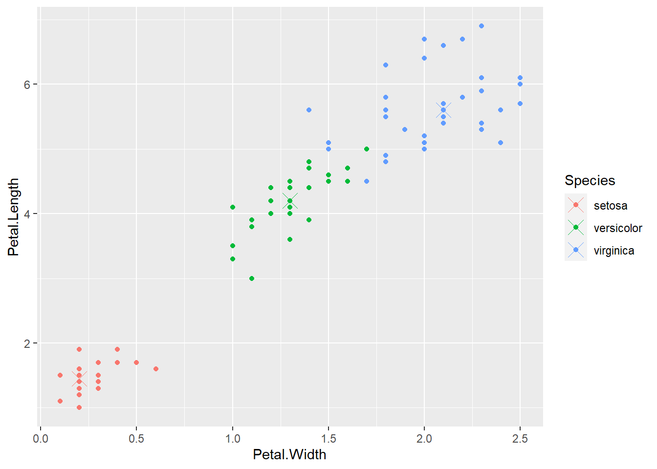
53.3 Predicting New Values
# Predict using our model built on the training set, on the testing set
pred <- predict(modFit, testing)

# Create a new variable corresponding to correct predictions
testing$predRight <- pred==testing$Species
table(pred, testing$Species)
##
## pred setosa versicolor virginica
## setosa 15 0 0
## versicolor 0 14 0
## virginica 0 1 15# View the incorrectly predicted classes
qplot(Petal.Width, Petal.Length, colour = predRight, data = testing, main = "New Data Predictions")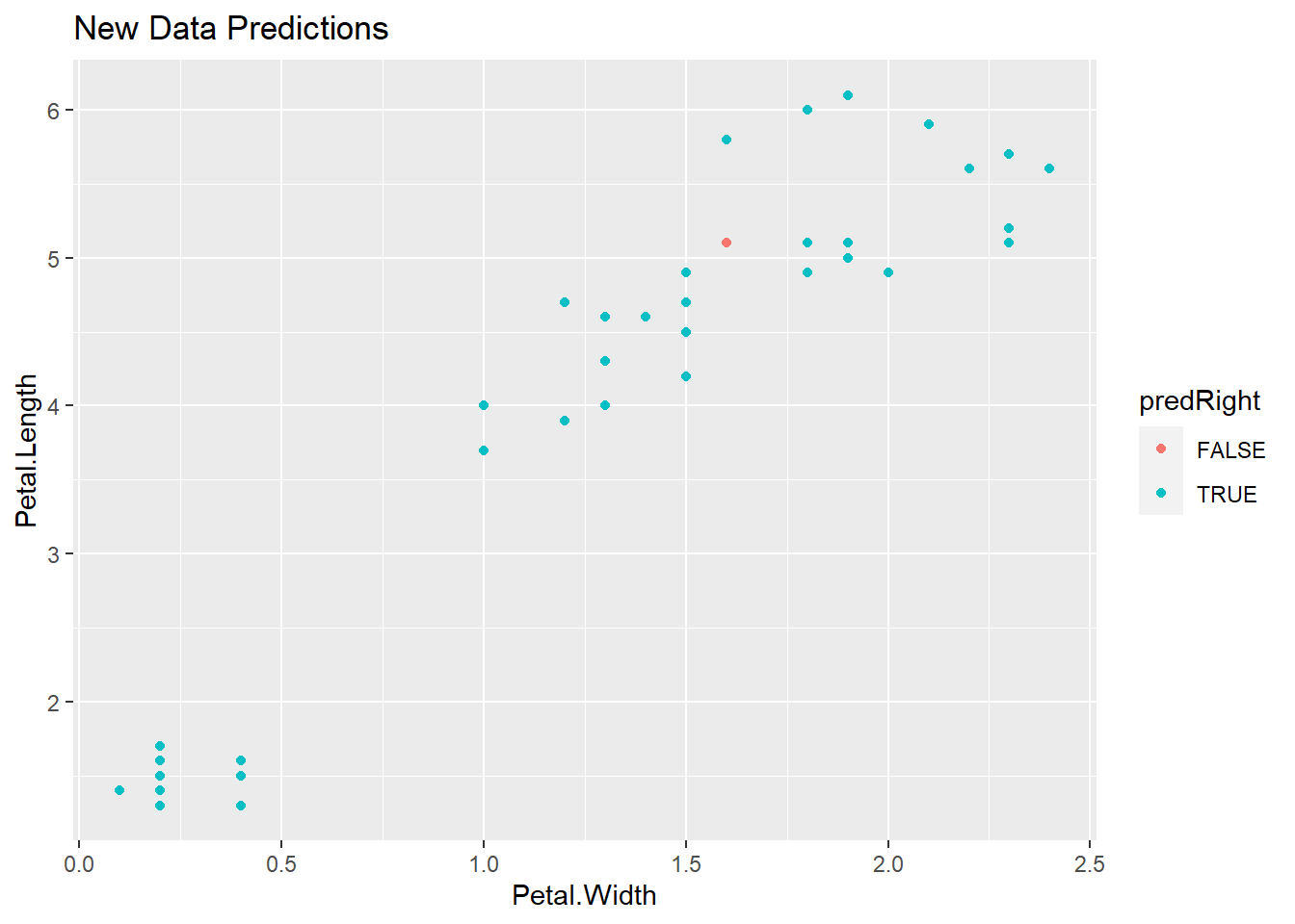
53.4 Notes
- Random forests are usually one of the two top performing algorithms along with boosting in prediction contests
- Random forests are difficult to interpret but often very accurate.
- Care should be taken to avoid overfitting.