58 Forecasting

58.1 Google Data: QuantMod

# Install package
library(quantmod); library(DT)

# Get trade information
from.dat <- as.Date("01/01/08", format = "%m/%d/%y")
to.dat <- as.Date("12/31/13", format = "%m/%d/%y")

getSymbols("GOOG", scr="google", from = from.dat, to = to.dat)

## [1] "GOOG"

head(GOOG)

##            GOOG.Open GOOG.High GOOG.Low GOOG.Close GOOG.Volume GOOG.Adjusted
## 2008-01-02  345.1413  347.3829 337.5996   341.3157     8646000      341.3157
## 2008-01-03  341.3505  342.1426 336.9969   341.3854     6529300      341.3854
## 2008-01-04  338.5759  339.2086 326.2770   327.2733    10759700      327.2733
## 2008-01-07  325.7490  329.9034 317.4850   323.4128    12854700      323.4128
## 2008-01-08  325.2808  328.7478 314.3218   314.6606    10718100      314.6606
## 2008-01-09  313.8436  325.4501 310.0927   325.3804    13529800      325.3804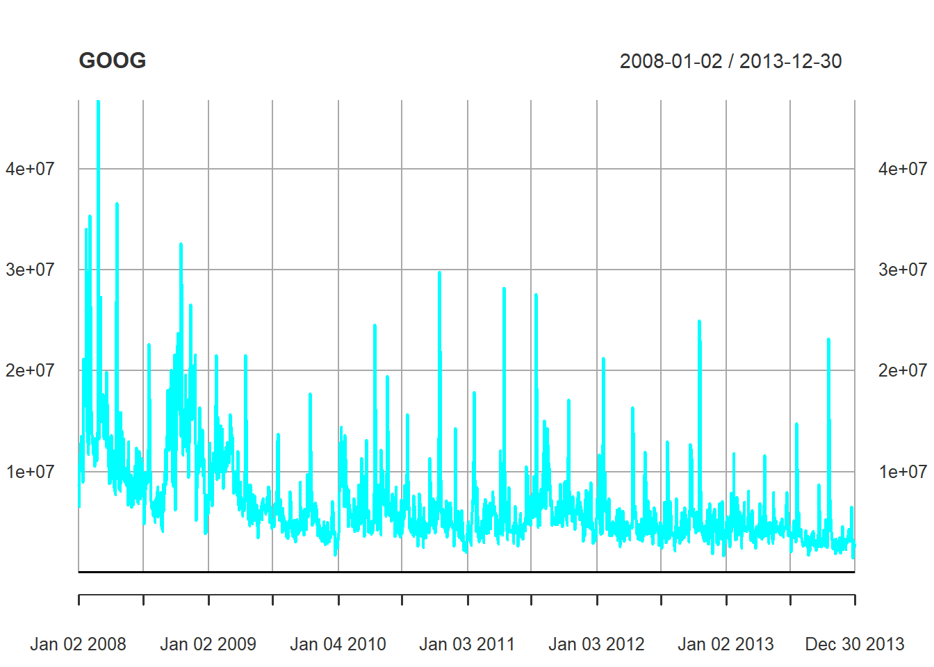

plot(GOOG)

# Summarise monthly and store as a time series 
mGoog <- to.monthly(GOOG)
googOpen <- Op(mGoog)
ts1 <- ts(googOpen, frequency = 12)
plot(ts1, xlab = "Years+1", ylab = "GOOG", col = "red")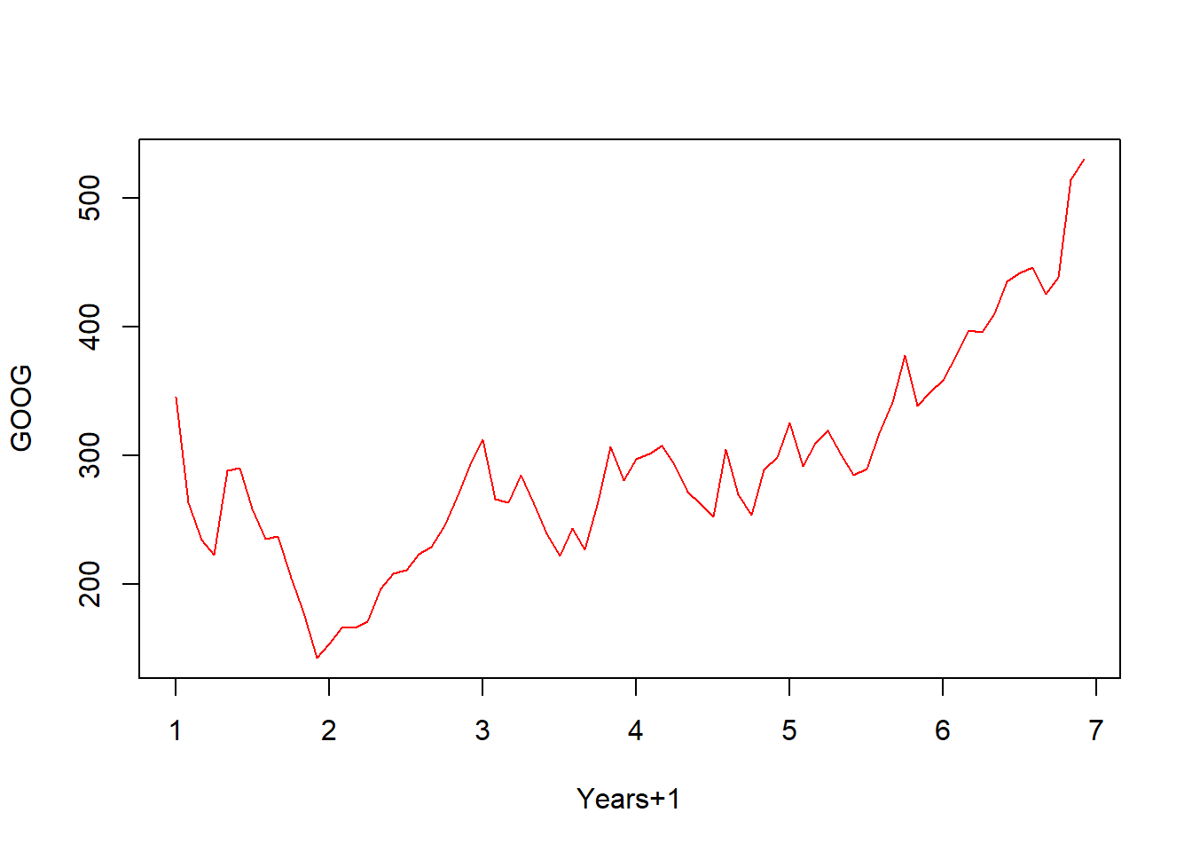

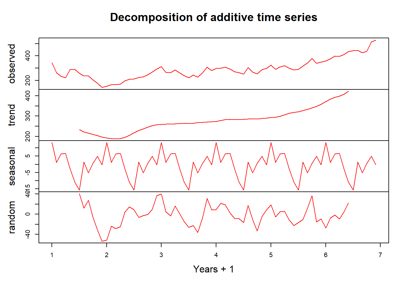
58.2 Example Time Series Decomposition

Trend - Consistently increasing pattern over time
Seasonal - When there is a patter over a fixed period of time that recurs
Cyclic - When data rises and falls over non fixed periods

Time series can be easily decomposed into parts using the decompose() function.

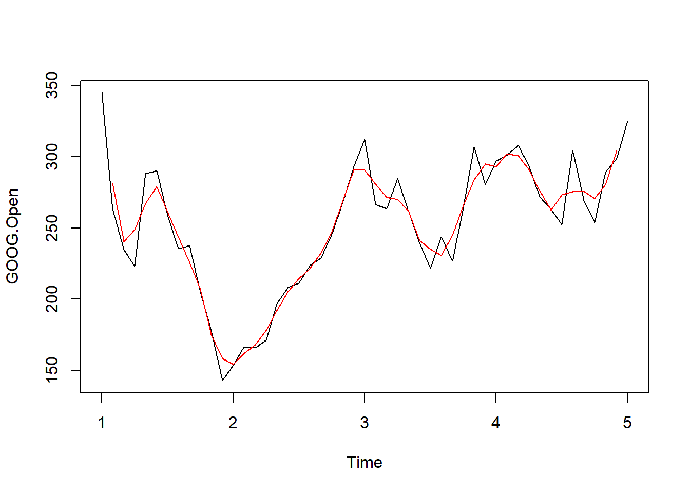
plot(decompose(ts1), xlab = "Years + 1", col = "red")

58.3 Training and Test Sets

In order to build training and test sets for these models, they must have consecutive time intervals. In the example below, we will use time intervals \(1 \rightarrow 5\).

ts1Train <- window(ts1, start = 1, end = 5)
ts1Test <- window(ts1, start = 5, end = (7-0.01))
ts1Train

##        Jan      Feb      Mar      Apr      May      Jun      Jul      Aug
## 1 345.1413 263.3479 234.8746 223.0340 288.0752 290.1624 258.8199 235.3728
## 2 153.7238 166.5208 166.0426 171.2481 196.7774 208.5832 211.3080 223.5322
## 3 312.3044 266.3018 263.6119 284.6082 262.2670 239.3180 221.8136 243.5820
## 4 297.1263 301.1163 307.7365 293.2807 271.8311 263.0341 252.4239 304.4688
## 5 325.2509                                                               
##        Sep      Oct      Nov      Dec
## 1 237.4948 204.8073 178.1224 142.8047
## 2 228.9817 245.5795 267.5372 292.9669
## 3 226.6405 264.0104 306.7154 280.4488
## 4 269.3654 253.9731 288.9669 298.8797
## 5

58.4 Simple Moving Average

One simple way to carry out forecasting is to perform a simple moving average. \[\hat{T_t} = \frac{1}{m} \sum_{j=-k}^k y_{t+j}\] where \(k = \frac{m-1}{2}\)

library(forecast)
plot(ts1Train)
lines(ma(ts1Train, order = 3), col = "red")

58.5 Exponential Smoothing

With exponential smoothing, near-by time points are weighted as higher values, or more heavily than time points that are farther away. So there’s a large number of different classes of smoothing models that you can choose. Simple exponential smoothing model: \[\hat{y}_{t+1} = \alpha y_t + (1-\alpha)\hat{y}_{t-1}\]

# Create the exponential smoothing data
ets1 <- ets(ts1Train, model="MMM")

# Forecast using this data
fcast <- forecast(ets1)

# Plot the results
plot(fcast, ylim = c(0, 1300))
lines(ts1Test, col = "red")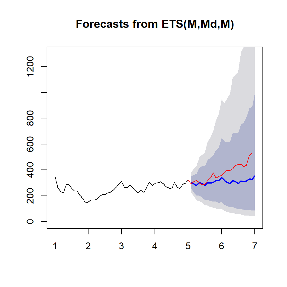

The accuracy of the forecasts can be calculated using the accuracy() function:

accuracy(fcast, ts1Test)

##                      ME     RMSE      MAE        MPE      MAPE      MASE
## Training set  0.2000302 26.09189 20.65928 -0.3572633  8.302526 0.3933832
## Test set     69.8911746 93.08104 72.04076 16.2879469 17.032408 1.3717625
##                       ACF1 Theil's U
## Training set -0.0002846501        NA
## Test set      0.7575349604  3.375609

58.6 Notes

Forecasting and timeseries prediction is an entire field
Rob Hyndman’s “Forecasting: Principals and Practice” is a good place to start
See quantmod and quandl packages fro finance-related problems

Cautions:

Be wary of spurious correlations
Be careful how far you predict (extrapolation)
Be wary of dependencies over time