23 Multivariable Regression Analysis
The general linear model extends simple linear regression by adding terms linearly into the model:
\[Y_i = \beta_1 X_1i + \beta_2 X_2i + ... + \beta_p X_pi + \epsilon_i = \sum_{k=1}^p X_{ik}\beta_j + \epsilon_i\]
- Here \(X_{1i} = 1\) generally, so that the intercept is included.
- Least squares (and hence ML estimates under iid Gaussianity of the errors) minimises:
\[\sum_{i=1}^n (Y_i - \sum_{k=1}^p X_{ki} \beta_j)^2\]
- Note, the important linearity is linearity in the coefficients, thus:
\[Y_i = \beta_1 X_{1i}^2 + \beta_2 X_{2i}^2 + ... + \beta_p X_{pi}^2 + \epsilon_i\]
- Still a linear model, we’ve only squared the elements of the predictors.
23.1 How to Get Estimates
Recall that the leats squares estimate for regression through the origin \[E[Y_i] = {{\sum X_i Y_i}\over{\sum X_i^2}}\]
- Lets consider two regressors, \(E[Y_i] = X_{1i} \beta_1 + X_{2i} \beta_2 = \mu_i\).
- Least squares tries to minimise:
\[\sum_{i=1}^n(Y_i - X_{1i} \beta_1 - X_{2i} \beta_2)^2\]
Starting with the formula for least squares, we can fix \(\beta_1\) and \(X_{i1}\) to get \(\tilde{y_i}\): \[\sum_{i=1}^n(Y_i - X_{1i} \beta_1 - X_{2i} \beta_2)^2\]
- Where: \[\tilde{y_i} = Y_i - X_{1i} \beta_1\] Leaves us with:
\[\sum_{i=1}^n(\tilde{y_i} - X_{2i} \beta_2)^2\]
Finding \(\tilde{y_i}\) can allow us to calculate \(\beta_2\): \[\beta_2 = {{\sum \tilde{y_i} X_{2i}}\over{\sum X_{2i}^2}}\] \[\sum_{i=1}^n(\tilde{y_i}- X_{2i} \beta_2)^2\]
23.2 Interprettion of the model coefficients wrt the model
So our model is essentially the sum of all of the regressors, multiplied by their slopes: \[E[Y|X_1 = x_1, ..., X_p = x_p] = \sum_{k=1}^p x_k \beta_k\] But what if we incremented one of the regressors by 1?
\[E[Y|X_1 = x_1 + 1, ..., X_p = x_p] = (x_1 + 1)\beta_1 + \sum_{k=1}^p x_k \beta_k\] So if we were to subtract these two terms from eachother:
\[E[Y|X_1 = x_1 + 1, ..., X_p = x_p] = - E[Y|X_1 = x_1, ..., X_p = x_p]\]
\[= (x_1 + 1)\beta_1 + \sum_{k=1}^p x_k \beta_k + \sum_{k=1}^p x_k \beta_k = \beta_1\]
This works out to be \(\beta_1\). What this effectively tells us, is that a multivariate regression coefficient is the expected change in the response per unit change in the regressor, holding all of the other regressors fixed.
This, in turn, effectively holds the other variables constant.
23.3 Fitted values, residuals and residual
All of our single linear regression qiantites can be extended to multiple linear models due to the magic of linear algebra.
- Model \(Y_i = \sum_{k=1}^p X_{ik}\beta_k + \epsilon_i\) where \(\epsilon_i \sim N(0, \sigma^2)\)
- Fitted responses \(\hat{Y_i} = \sum_{k=1}^p X_{ik} \hat{\beta_k}\)
- Residuals \(e_i = Y_i - \hat{Y_i}\)
- Variance estimate \(\hat{\sigma^2} = {1\over{n-p}} \sum_{i=1}^n e_i^2\) so here, it’s a bit different, as we’re dividing by n-p instead of n-2 as we’re using p number of regressors, the degrees of freedom will change.
23.4 Multivariable Regression Examples
# Lets now examine more closely the relationship between fertility and the rest of the variables with multiple regression without any wieghts or square terms
summary(lm(Fertility ~. , data = swiss))
##
## Call:
## lm(formula = Fertility ~ ., data = swiss)
##
## Residuals:
## Min 1Q Median 3Q Max
## -15.2743 -5.2617 0.5032 4.1198 15.3213
##
## Coefficients:
## Estimate Std. Error t value Pr(>|t|)
## (Intercept) 66.91518 10.70604 6.250 1.91e-07 ***
## Agriculture -0.17211 0.07030 -2.448 0.01873 *
## Examination -0.25801 0.25388 -1.016 0.31546
## Education -0.87094 0.18303 -4.758 2.43e-05 ***
## Catholic 0.10412 0.03526 2.953 0.00519 **
## Infant.Mortality 1.07705 0.38172 2.822 0.00734 **
## ---
## Signif. codes: 0 '***' 0.001 '**' 0.01 '*' 0.05 '.' 0.1 ' ' 1
##
## Residual standard error: 7.165 on 41 degrees of freedom
## Multiple R-squared: 0.7067, Adjusted R-squared: 0.671
## F-statistic: 19.76 on 5 and 41 DF, p-value: 5.594e-10Here, the -0.17 estimate for the slope term for the Agriculture variable, means that our model estimates an expected 0.17 decrease (slope is negative) in standardised fertility for every 1% increase in percentage of males involved in agriculture in holding the remaining variables constant.
The 0.07030 Std. Error refers to how precise that variable is.
If we wanted to perform a hypothesis test as to whether the slope of the agriculture term is 0 or not;
\(H_0 : \beta_{Agri} = 0\) vs \(H_A : \beta_{Agri} \ne 0\)
We would take the estimate, minus the hypothesised value, which in this case is 0, then divide it by the standard error:
\[ t-value= {{-0.17211}\over{0.07030}} = -2.448\]
How does this compare to a model that explains fertility only using the agriculture variable?
##               Estimate Std. Error   t value     Pr(>|t|)
## (Intercept) 60.3043752 4.25125562 14.185074 3.216304e-18
## Agriculture  0.1942017 0.07671176  2.531577 1.491720e-02
The magnitude of the slope here is almost the same, 0.19 instead of 0,17, however the sign of the slope has now changed. Adjusting for the other variables has changed the sign of this term in the case of our multiple regression model. This is an example of Simpson’s percieved paradox. In both cases, the agriculture variable is strongly statistically significant.
23.5 Dummy Variables are Smart
Consider a linear model wherein each \(X_i\) is binary, so that it is a 1, if measurement \(i\) is in a group and 0 otherwise.
- Then for people in the group \(E[Y_i] = \beta_0 + \beta_1\)
- And for people not in the group \(E[Y_i] = \beta_0\)
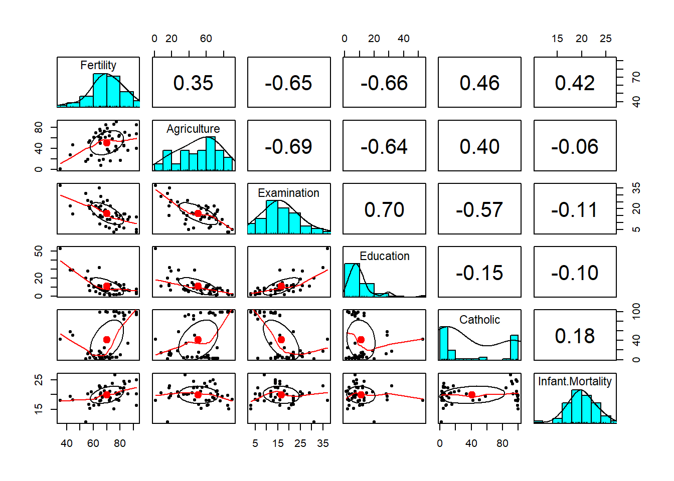
23.6 More Multivariable Regression Examples
##              Fertility Agriculture Examination Education Catholic
## Courtelary        80.2        17.0          15        12     9.96
## Delemont          83.1        45.1           6         9    84.84
## Franches-Mnt      92.5        39.7           5         5    93.40
## Moutier           85.8        36.5          12         7    33.77
## Neuveville        76.9        43.5          17        15     5.16
## Porrentruy        76.1        35.3           9         7    90.57
##              Infant.Mortality
## Courtelary               22.2
## Delemont                 22.2
## Franches-Mnt             20.2
## Moutier                  20.3
## Neuveville               20.6
## Porrentruy               26.6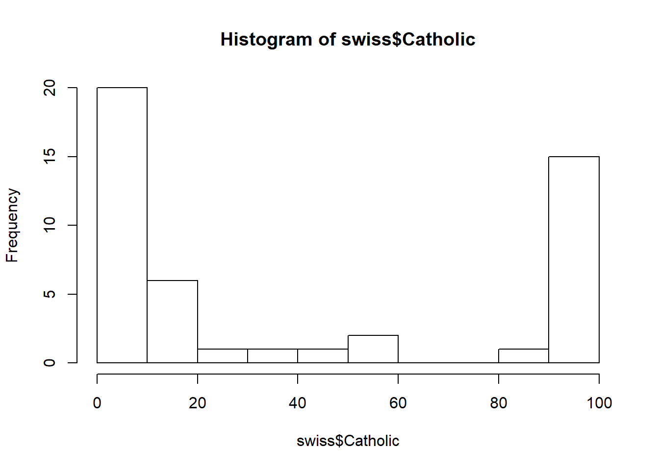
# Make a catholic binary variable if the province is majority catholic or not

swiss = mutate(swiss, CatholicBin = 1 * (Catholic > 50))
head(swiss)
## Fertility Agriculture Examination Education Catholic Infant.Mortality
## 1 80.2 17.0 15 12 9.96 22.2
## 2 83.1 45.1 6 9 84.84 22.2
## 3 92.5 39.7 5 5 93.40 20.2
## 4 85.8 36.5 12 7 33.77 20.3
## 5 76.9 43.5 17 15 5.16 20.6
## 6 76.1 35.3 9 7 90.57 26.6
## CatholicBin
## 1 0
## 2 1
## 3 1
## 4 0
## 5 0
## 6 1g <- ggplot(swiss, aes(x = Agriculture, y = Fertility, colour = CatholicBin)) +
geom_point() +
xlab("% in Agriculture") +
ylab("Fertility")
g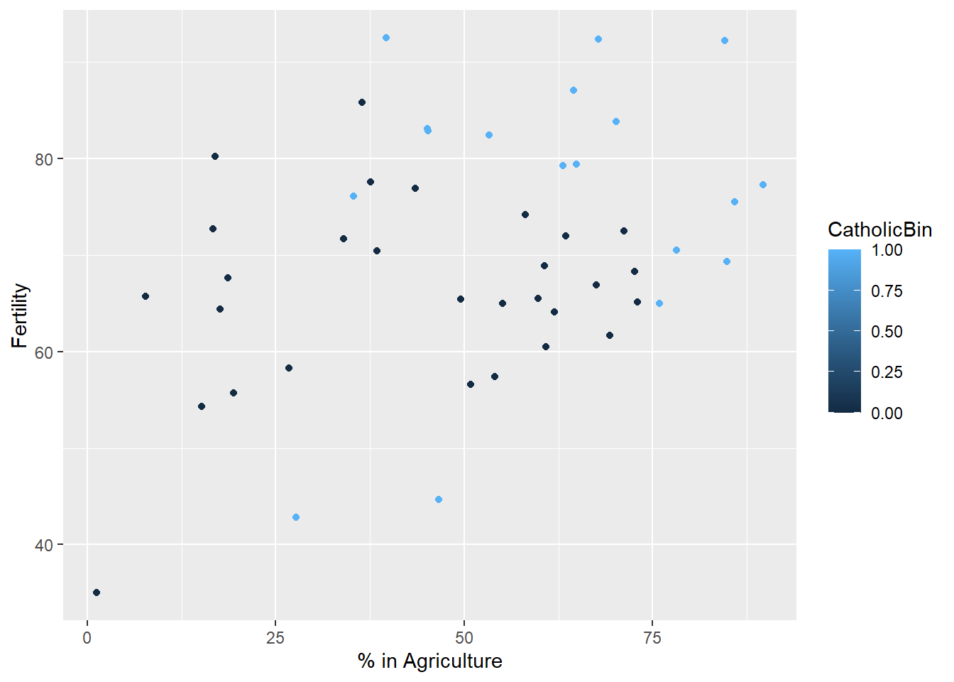
Our first model will be \(E[y|x_1x_2] = \beta_0 + \beta_1 x_1\) where y = fertility, x1 = agriculture and x2 = 1 or 0 if the majority porvince is catholic or not.
Our second modle will be \(E[y|x_1x_2] = \beta_0 + \beta_1 x_1 + \beta_2 x_2\), in the event that x = 0, the model is reduced to model 1. However, if the value of x2 is 1, the model will \(E[y|x_1x_2] = \beta_0 +\beta_2 +\beta_1 x_1\). Fitting this model will effectively fit two models, both with the same slope term \(\beta_1\) but both will have different intercepts.
Lets consider a third model. \(E[y|x_1x_2] = \beta_0 + \beta_1 x_1 + \beta_2 x_2 + \beta_3 x_1 x_2\). When x2 = 0 in this case, this model is reduced to be that of model 1. When x2 = 1, we are left with \(E[y|x_1x_2] = (\beta_0 + \beta_2)+(\beta_1+ \beta_3)x_1\).
So if we include an interaction term, then we fit two lines, but now these two lines will have different slopes as well.
- Interaction term -> two lines, different slopes, diferent intercepts
- No interaction term binary variable -> two lines, two intercepts, same slope.
So first, lets just plot a model that does not inclue religeon:
model = lm(Fertility ~ Agriculture, data = swiss)
g1 = g
g1 <- g1 + geom_abline(intercept = coef(model)[1], slope = coef(model)[2], size = 2)
g1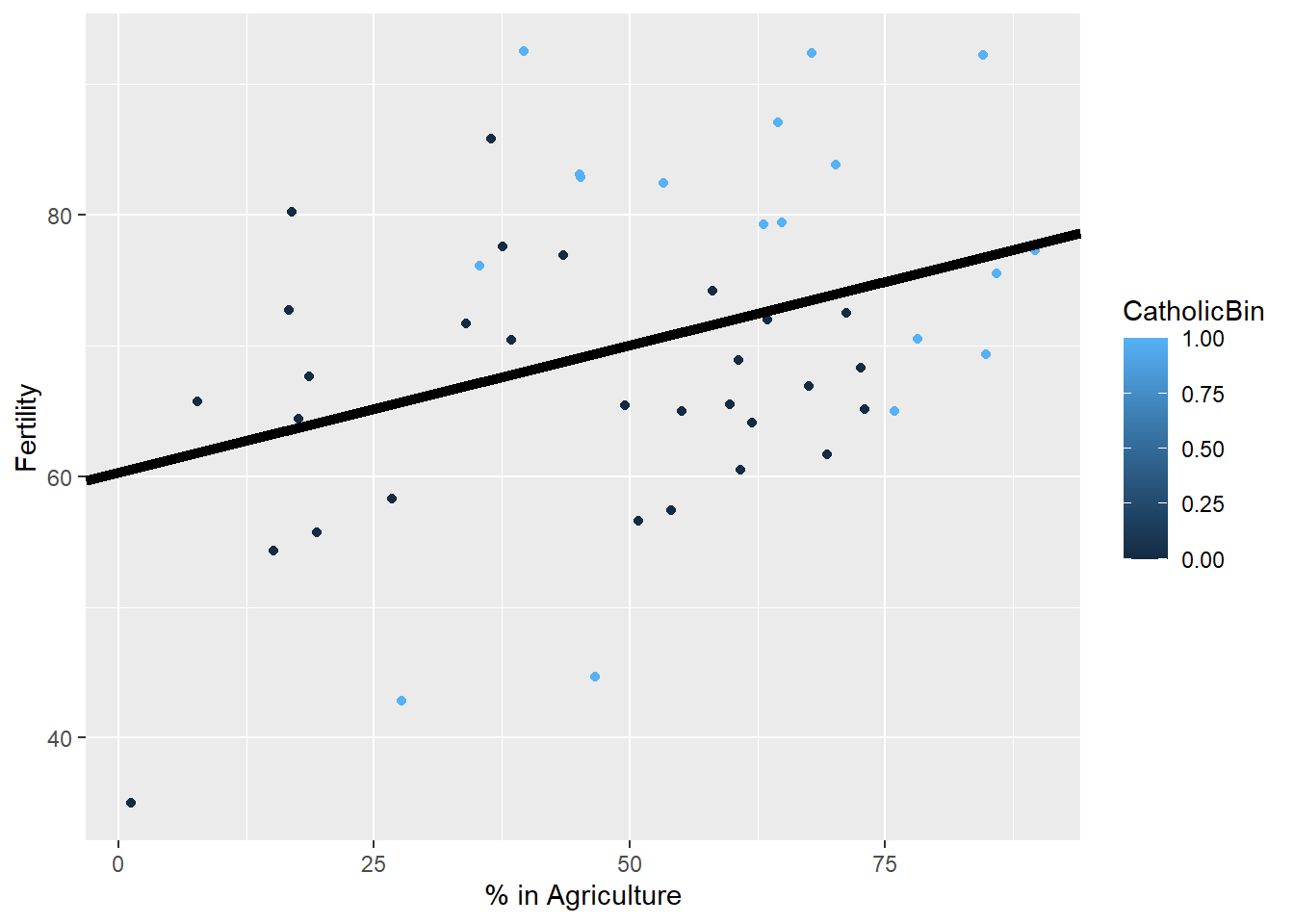
23.6.1 Two lines, two intercepts
##                        Estimate Std. Error   t value     Pr(>|t|)
## (Intercept)          60.8322366  4.1058630 14.815944 1.032493e-18
## Agriculture           0.1241776  0.0810977  1.531210 1.328763e-01
## factor(CatholicBin)1  7.8843292  3.7483622  2.103406 4.118221e-02
g1 = g
g1 <- g1 + geom_abline(intercept = coef(model)[1], slope = coef(model)[2])
g1 <- g1 + geom_abline(intercept = coef(model)[1] + coef(model)[3], slope = coef(model)[2])
g1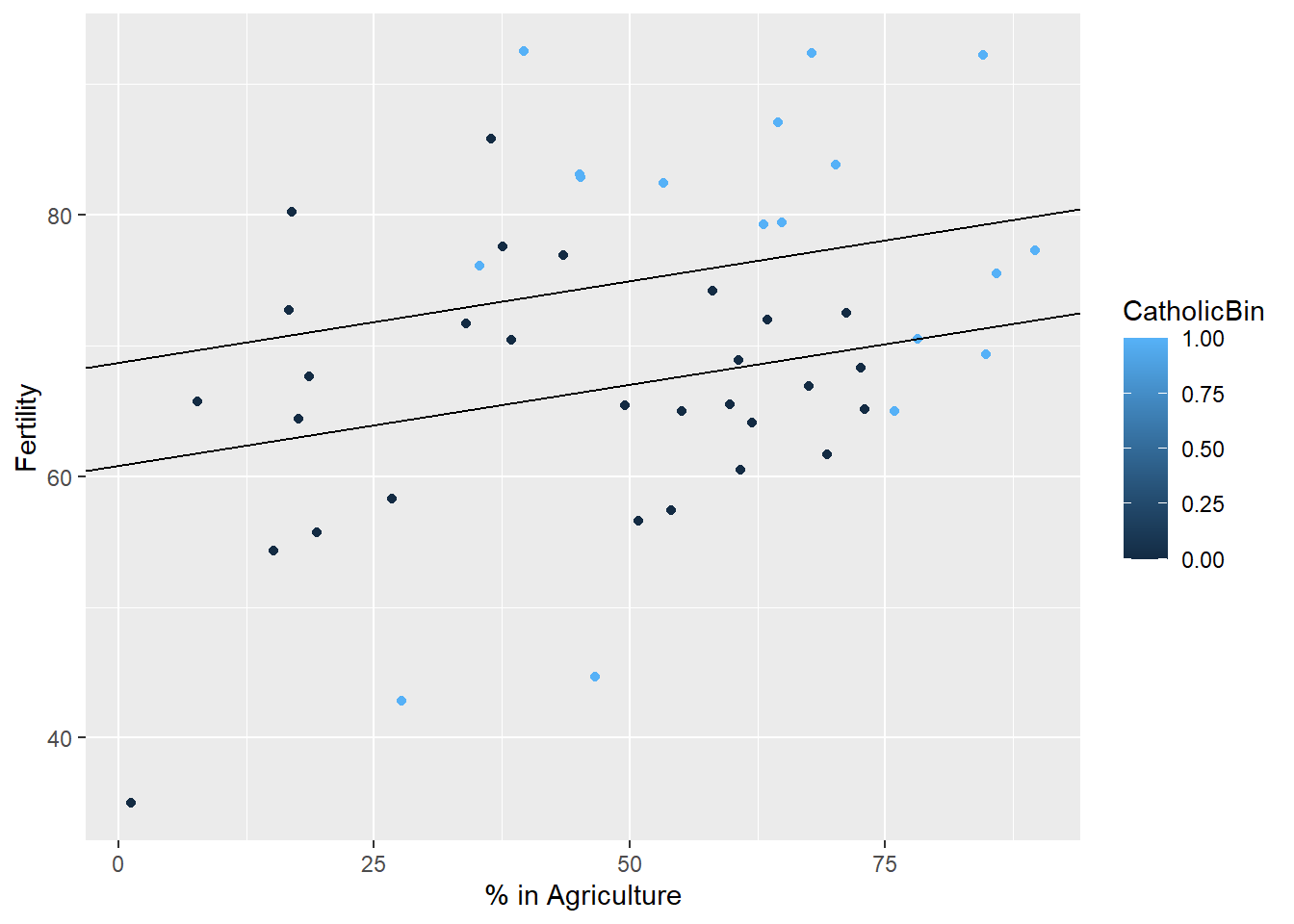
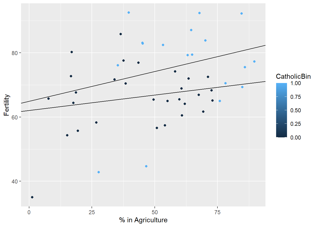
23.6.2 Interaction term: Two lines, two slopes, two intercepts
model <- lm(Fertility ~ Agriculture * factor(CatholicBin), data = swiss)
summary(model)$coefficients
## Estimate Std. Error t value
## (Intercept) 62.04993019 4.78915566 12.9563402
## Agriculture 0.09611572 0.09881204 0.9727127
## factor(CatholicBin)1 2.85770359 10.62644275 0.2689238
## Agriculture:factor(CatholicBin)1 0.08913512 0.17610660 0.5061430
## Pr(>|t|)
## (Intercept) 1.919379e-16
## Agriculture 3.361364e-01
## factor(CatholicBin)1 7.892745e-01
## Agriculture:factor(CatholicBin)1 6.153416e-01g1 = g
g1 <- g1 + geom_abline(intercept = coef(model)[1], slope = coef(model)[2]) +
geom_abline(intercept = coef(model)[1] + coef(model)[3], slope = coef(model)[2] + coef(model)[4])
g1