13 Multiple Comparisons

13.1 Multiple Testing

13.1.1 Key Ideas

Hypothesis testing / significance analysis is commonly overused
Correcting for multiple testing avoids false positives or discoveries
Two key components
- Error measure
- Correction

13.1.2 Why Correct for Multiple Tests?

If we perform tests with an alpha value of \(5\%\), meaning that we have a \(5\%\) chance of our finding happening by chance, then we go away and test 20 different hypotheses, then it becomes extremely likely that at least one of them would result in a coincidence.

Here, it becomes necessary to point out that p values and hypothesis tests are not interchangeable.

13.2 Error Rates

False positive rate

The rate at which false results \((\beta=0)\) are called significant \(E [\frac{V}{m_0}]\)

Family wise error rate (FWER)

The probability of at least one false positive \(Pr(V\ge1)\)

False discovery rate (FDR)

The rate at which claims of significance are false \(E [\frac{V}{R}]\)

13.3 Controlling the False Positive Rate

If P-values are correctly calculated calling all \(P < \alpha\) significant will control the false positive rate at level \(\alpha\) on average.

Problem: suppose that you perform 10,000 tests and \(\beta = 0\) for all of them. * Suppose that you call \(P < 0.05\) significant. * The expected number of false positives is: \(10,000 \times 0.05 = 500\) false positives. * How do we avoid so many false positives?

13.3.1 Controlling the Family-wise Error Rate

The Biferroni Correction is the oldest multiple testing correction.

Basic Idea:

Suppose you do \(m\) tests
You want to control FWER at level \(\alpha\) so \(Pr(V\ge1) < \alpha\)
Calculate P-Values normally
Set \(\alpha_{fwer} = \frac{\alpha}{m}\)
Call all P-values less than \(\alpha_{fwer}\) significant

Pros: Easy to calculate Cons: May be very conservative

13.3.2 Controlling the False Discovery Rate (FDR)

This is the most popular correction when performing lots of tests, say in genomics, imaging, astronomy, or other signal-pressing disciplines.

Basic idea:

Suppose that you do \(m\) tests.
You want to control FDR at level \(\alpha\) so \(E[\frac{V}{R}]\)
Calculate P-values normally
Order the P values from smallest to largest \(P_{[1]}, P_{[2]}, P_{[3]}...P_{[m]}\)
Call any \(P_{[i]} \le \alpha \times \frac{i}{m}\) significant

Pros: Still pretty easy to calculate, less conservative (maybe much less) Cons: Allows for more false positives, may behave strangely under dependence

13.4 Adjusted P-Values

One approach is to adjust the threshold \(\alpha\)
A different approach is to calculate “adjusted p-values”
These are no longer p-values
Theses can however, be used directly without adjusting \(\alpha\)

Example:

Suppose that P-values are \(P_{[1]}, P_{[2]}, P_{[3]}...P_{[m]}\)
You could adjust them by taking \(P_{i}^{fwer}=max(m)\times P_i, 1\) for each P-value
Then if you call all \(P_{i}^{fwer} < \alpha\) significant, you will control the FWER

13.5 Case Study 1: No True Positives

The code below will create 1000 linear models using random normally distributed data with no underlying relationship. We’ll record the p-values for each regression coefficient and see how many times we falsely detect a statistically significant relationship.

We’ll then look at different ways that we can adjust the p-values to mitigate these errors.

set.seed(1234)

pValues <- rep(NA, 1000)

# We're going to simulate linear models for totally unrelated data 1000 times
for(i in 1:1000){
  y <- rnorm(20)
  x <- rnorm(20)
  
  # This will grab the p values for the coefficients for totally unrelated variables
  pValues[i] <- summary(lm(y ~ x))$coeff[2, 4]
}

# In none of these cases was there a single meaningful relationship
# However, there are still 47 cases with statistically significant p-values
sum(pValues < 0.05)

## [1] 47

## So what happens if we adjust the p-values?

# This will control for FWER
sum(p.adjust(pValues, method = "bonferroni") < 0.05)

## [1] 0

# This controls for FDR
sum(p.adjust(pValues, method = "BH") < 0.05)

## [1] 0

13.6 Case Study 2: 50% True Positives

set.seed(1234)

pValues <- rep(NA, 1000)

# We're going to simulate linear models for totally unrelated data 1000 times
for(i in 1:1000){
  y <- rnorm(20)
  x <- rnorm(20)
  
  # First 500 beta= 0, last 500 beta = 2
  if(i <= 500){y <- rnorm(20)}else{y <- rnorm(20, mean = 2*x)}
  
  # This will grab the p values for the coefficients for totally unrelated variables
  pValues[i] <- summary(lm(y ~ x))$coeff[2, 4]
}

trueStatus <- rep(c("zero", "not zero"), each = 500)
table(pValues < 0.05, trueStatus)

##        trueStatus
##         not zero zero
##   FALSE        0  478
##   TRUE       500   22

# This controls for FWER
table(p.adjust(pValues, method = "bonferroni") < 0.05, trueStatus)

##        trueStatus
##         not zero zero
##   FALSE       13  499
##   TRUE       487    1

# This controls for FDR
table(p.adjust(pValues, method = "BH") < 0.05, trueStatus)

##        trueStatus
##         not zero zero
##   FALSE        0  488
##   TRUE       500   12

P values vs Adjusted P values

par(mfrow = c(1,2))
plot(pValues, p.adjust(pValues, method = "bonferroni"), pch=19)
plot(pValues, p.adjust(pValues, method = "BH"), pch=19)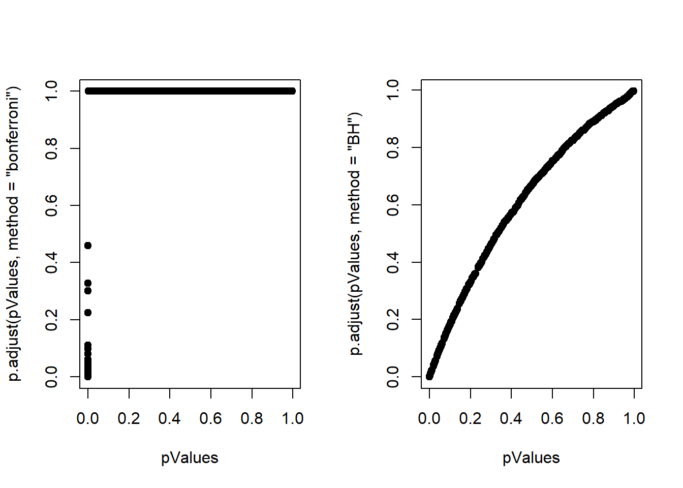

13.7 Notes

Multiple testing is an entire sub field
A basic Bonferroni/BH correction is usually good enough
If there is a strong dependence between tests, there may be problems
- Consider method = “BY”