24 Adjustment

Adjustment is when new regressors are added inot a linear model to investigate the role of a third variable on the relationship between another two, as a Third variable can often distort or confound relationships between two other regressors.

The general rule for any model is garbage in -> garbage out, for example, measuring breath mint usage in a lung cancer data set. If those who smoke will more often than not have more of a reason to use breath mints, purely from a data stand point there would be expected, a strong correlation between breath mint usage and lung cancer.

If you have found a strong relationship between cancer an breath mint usage, how would you defend your finding against the accusation that it’s just variability in smoking habits?

If your finding held up against both smokers and non smokers when analyzed separately, you might have something. This is the idea of adding a regression variable into a model as adjustment.

24.1 Coefficient of interest

The coefficient of interest is interpreted as the effect of the predictor on the response, holding the adjustment variable constant.

24.2 Adjustment examples

24.2.1 Simulation 1:

n <- 100; t <- rep(c(0, 1), c(n/2, n/2)); x <- c(runif(n/2), runif(n/2));
beta0 <- 0; beta1 <- 2; tau <- 1; sigma <- .2
y <- beta0 + x * beta1 + t * tau + rnorm(n, sd = sigma)
plot(x, y, type = "n", frame = FALSE)
abline(lm(y ~ x), lwd = 2)
abline(h = mean(y[1 : (n/2)]), lwd = 3)
abline(h = mean(y[(n/2 + 1) : n]), lwd = 3)
fit <- lm(y ~ x + t)
abline(coef(fit)[1], coef(fit)[2], lwd = 3)
abline(coef(fit)[1] + coef(fit)[3], coef(fit)[2], lwd = 3)
points(x[1 : (n/2)], y[1 : (n/2)], pch = 21, col = "black", bg = "lightblue", cex = 2)
points(x[(n/2 + 1) : n], y[(n/2 + 1) : n], pch = 21, col = "black", bg = "salmon", cex = 2)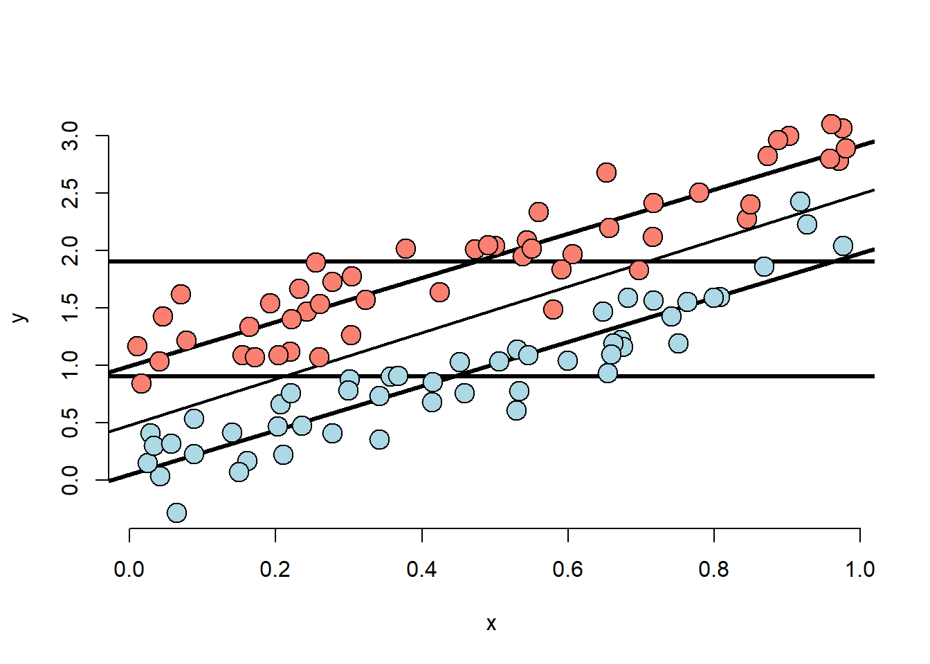

• The X variable is unrelated to group status
• The X variable is related to Y, but the intercept depends on group status.
• The group variable is related to Y.
  • The relationship between group status and Y is constant depending on X.
  • The relationship between group and Y disregarding X is about the same as holding X constant

24.2.2 Simulation 2:

n <- 100; t <- rep(c(0, 1), c(n/2, n/2)); x <- c(runif(n/2), 1.5 + runif(n/2));
beta0 <- 0; beta1 <- 2; tau <- 0; sigma <- .2
y <- beta0 + x * beta1 + t * tau + rnorm(n, sd = sigma)
plot(x, y, type = "n", frame = FALSE)
abline(lm(y ~ x), lwd = 2)
abline(h = mean(y[1 : (n/2)]), lwd = 3)
abline(h = mean(y[(n/2 + 1) : n]), lwd = 3)
fit <- lm(y ~ x + t)
abline(coef(fit)[1], coef(fit)[2], lwd = 3)
abline(coef(fit)[1] + coef(fit)[3], coef(fit)[2], lwd = 3)
points(x[1 : (n/2)], y[1 : (n/2)], pch = 21, col = "black", bg = "lightblue", cex = 2)
points(x[(n/2 + 1) : n], y[(n/2 + 1) : n], pch = 21, col = "black", bg = "salmon", cex = 2)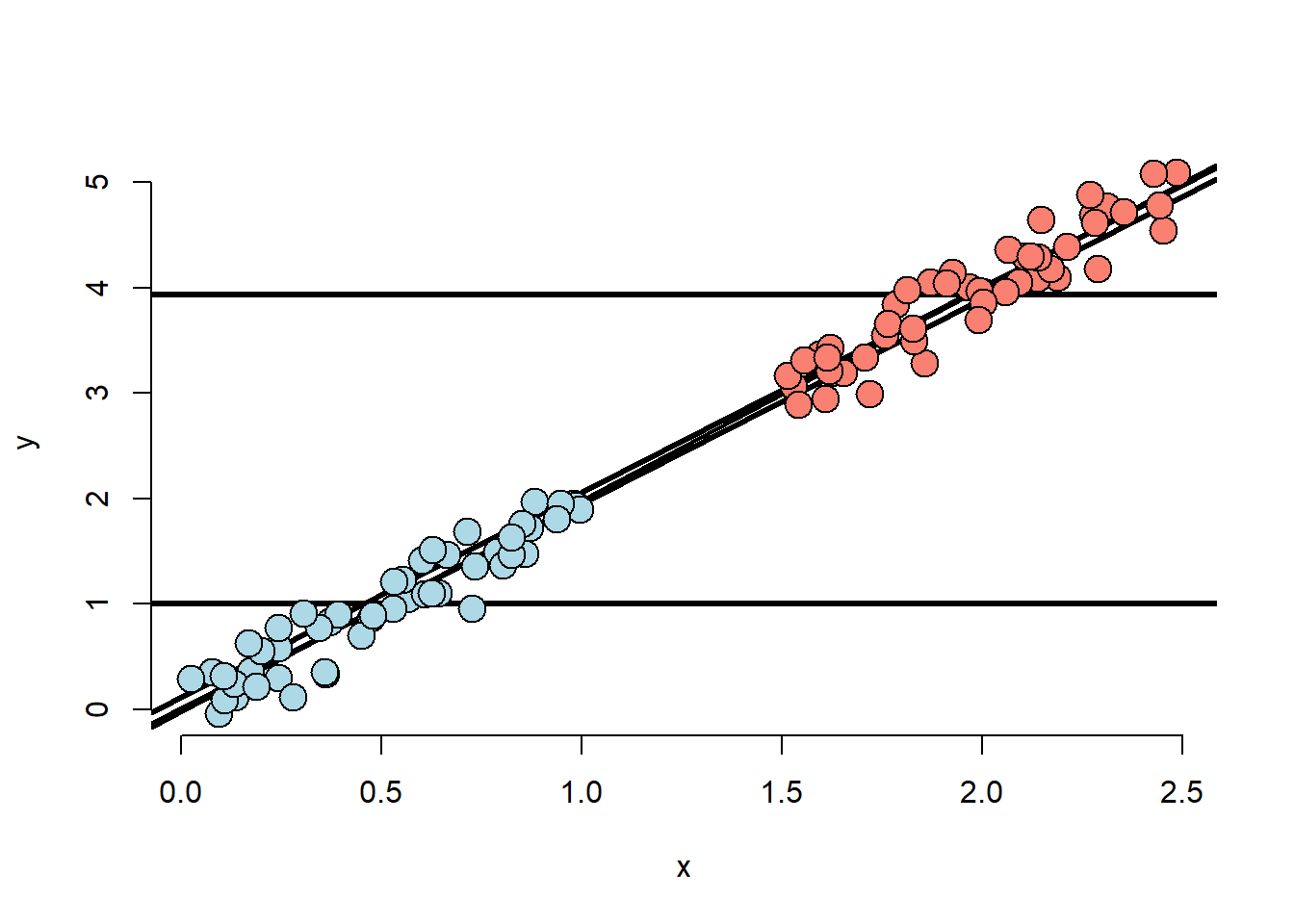

• The X variable is highly related to group status
• The X variable is related to Y, the intercept doesn’t depend on the group variable.
  • The X variable remains related to Y holding group status constant
• The group variable is marginally related to Y disregarding X.
• The model would estimate no adjusted effect due to group.
  • There isn’t any data to inform the relationship between group and Y.
  • This conclusion is entirely based on the model.

24.2.3 Simulation 3:

n <- 100; t <- rep(c(0, 1), c(n/2, n/2)); x <- c(runif(n/2), .9 + runif(n/2));
beta0 <- 0; beta1 <- 2; tau <- -1; sigma <- .2
y <- beta0 + x * beta1 + t * tau + rnorm(n, sd = sigma)
plot(x, y, type = "n", frame = FALSE)
abline(lm(y ~ x), lwd = 2)
abline(h = mean(y[1 : (n/2)]), lwd = 3)
abline(h = mean(y[(n/2 + 1) : n]), lwd = 3)
fit <- lm(y ~ x + t)
abline(coef(fit)[1], coef(fit)[2], lwd = 3)
abline(coef(fit)[1] + coef(fit)[3], coef(fit)[2], lwd = 3)
points(x[1 : (n/2)], y[1 : (n/2)], pch = 21, col = "black", bg = "lightblue", cex = 2)
points(x[(n/2 + 1) : n], y[(n/2 + 1) : n], pch = 21, col = "black", bg = "salmon", cex = 2)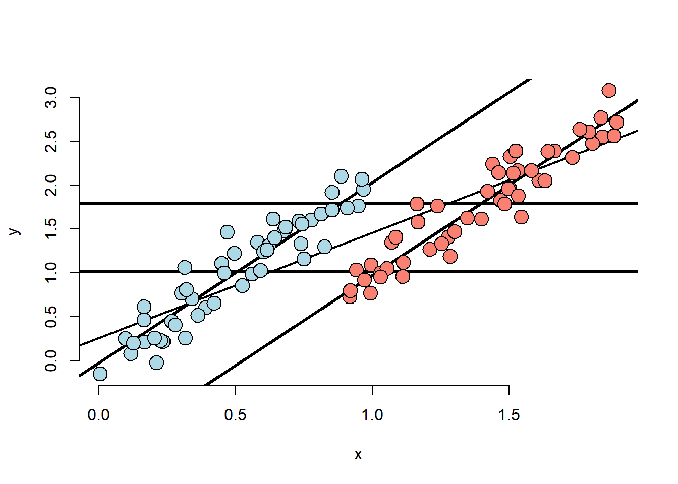

• Marginal association has red group higher than blue.
• Adjusted relationship has blue group higher than red.
• Group status related to X.
• There is some direct evidence for comparing red and blue holding X fixed.

p <- 1
n <- 100 
x2 <- runif(n)
x1 <- p * runif(n) - (1-p) * x2
beta0 <- 0
beta1 <- 1
tau <- 4
sigma <- .01
y <- beta0 + x1*beta1 + tau * x2 + rnorm(n, sd = sigma)

plot(x1, y, type = "n", frame = FALSE)
abline(lm(y~x1), lwd = 2)
co.pal <- heat.colors(n)
points(x1, y, pch = 21, col = "black", bg = co.pal[round((n-1)*x2+1)], cex = 2)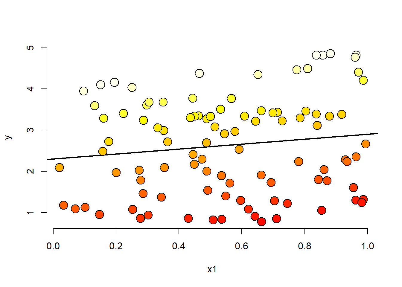

library(rgl)
plot3d(x1, x2, y)

24.3 Final thoughts

• Modelling multivariate relationships are hard
• Play around with simulaions to see how the inclusion o eclusion of another variable can change analyses
• The results of these anlyses deal with the impact of variables on assocations
  • Ascertaining mechanisms or cause are difficult subjects to be added on top of difficulty in understanding multivariate associations